
Copyright © 2026, Molsoft LLC
Jan 21 2026
Google Search:
Keyword Search:| Prev | ICM Language Reference Tables | Next |
[ CONSENSUS | CONSENSUSCOLOR | FILTER | FTP | GRAPHICS | GRID | GROB | GUI | IMAGE | LIBRARY | OBJECT | PLOT | SITE | TOOLS | WEBLINK | WEBAUTOLINK ]
The following predefined icm-shell tables are collections of different icm shell objects related to a certain topic. Note that these tables (as opposed to user-defined ICM tables ) usually only have the header section. You can show and list them. You can also change any table element by the usual icm assignment:Examples:
 IMAGE.color = yes       # this member is a logical
 IMAGE.stereoBase = 2.5  # redefine real distance between stereo panels
CONSENSUS |
The consensus symbol is established if the percentage of specified residues in a give column exceeds the fraction given in the 2nd column. In rows were we provide two symbols (e.g. "-n"), the first (e.g. '-') is used in alignment representations, while the letter form of this symbol (e.g. 'n') is used in residue selections, (e.g. a_/Cn ) The first matched consensus condition takes precedence. In an example below, if Q is found in more than 85% or sequences, its consensus symbol is Q, if the percentage is between 60 and 85, the symbol becomes q, and if no consensus is establish, the symbol becomes the dot character ('.').
#>T CONSENSUS
#>-symbol------fraction----residues---
   A           85          A
   C           85          C
   Q           85          Q
...
   d           60          ND
   -n          70          ED
   +o          60          RK
   gj          60          G
   q           70          Q
   p           60          P
   t           60          TSN
   "#h"        85          WLVIMAFCYHP
   %f          65          WLVIMAFCYHP
   " g"        85          -
See also: CONSENSUSCOLOR , CONSENSUS_strength , color alignment rs_ , ribbonColorStyle .
CONSENSUSCOLOR |
contains coloring schemes of residues according a multiple sequence alignment (see the align command). This table is saved together with the GUI preferences. Residue color is defined by two factors: its type, as listed in the first column of the table, AND the consensus character under which this residue is aligned. The consensus symbols are defined by the CONSENSUS table and are listed in the third column of the CONSENSUSCOLOR table that is loaded from the $ICMHOME/CONSENSUSCOLOR.tab file. In this scheme the same residue can be colored differently depending on the alignment in a current position.
#>T CONSENSUSCOLOR
#>-residue-----color-------symbols----
   *           *           *         # separator between sections
   ED          "#ff0000"   "-EDp"    # E and D residues will be colored red under '-','E' or 'D'
   KR          "#0000ff"   "+KRp"
See also: CONSENSUSCOLOR , CONSENSUS_strength , color alignment rs_ , ribbonColorStyle , set color.
FILTER |
[ FILTER.Z | FILTER.gz | FILTER.uue ]
contains filters which can be applied to the input stream in the read command. Components have names corresponding to standard file name extensions; their string value is a unix filter. Token %s is a placeholder for the file name. The provided defaults can be redefined in your _startup file. You can also add your own extensions and filters by doing the following:z = "pcat %s" # define the action for the unix packed files group table append FILTER header z # append new filter to the structureThe mechanism ICM employs allows one to keep the transformed files intact and avoid creating temporary files when possible (e.g. uuencode unix command always creates an output file). Existing extensions and defaults are given below. You may need to redefine the defaults by adding the exact path to the utility or using alternatives.
FILTER.Z |
allows you to read the compressed files (*.Z) directly leaving the compressed file intact. The default value: "zcat %s" . If you do not have zcat utility, try
FILTER.Z = "uncompress -c %s"
FILTER.gz |
The default value is "gunzip -c %s" .
FILTER.uue |
The default value is
"sed 's:begin .*:begin 600 /tmp/UUPtm:' %s | uudecode && cat /tmp/UUPtm && rm -f /tmp/UUPtm"This works for UNIX file system, write your own on the PC, if needed.
FTP |
[ FTP.createFile | FTP.keepFile | FTP.proxy | HTTP.proxy | HTTP.ignoreProxyDomains ]
table which controls reading from ftp.FTP.createFile |
(default no ). This flag is not active yet. The file is always created in the s_tempDir directory.
FTP.keepFile |
(default no ). If yes, the temporary file is kept in the s_tempDir directory. Otherwise the file is deleted.
FTP.proxy |
string name of the proxy server for ftp connections through firewall. Default: "" (empty string).
String format: ftp.proxy.host.com[:port]
HTTP.proxy |
string name of the proxy server for http connections through firewall. Default: "" (empty string).
String format: [user[:pass]@]http.proxy.host.com[:port]
HTTP.ignoreProxyDomains |
string with ';' separated list of domains where HTTP.proxy should not be used.
Example:
HTTP.ignoreProxyDomains = "localhost;*.molsoft.com" # local host + everything which ends with .molsoft.com
GRAPHICS |
[ GRAPHICS.alignmentRainbow | GRAPHICS.atomLabelShift | GRAPHICS.atomValueCircles | GRAPHICS.ballRadius | GRAPHICS.ballStickRatio | GRAPHICS.clashWidth | GRAPHICS.chainBreakStyle | GRAPHICS.chainBreakLabelDisplay | GRAPHICS.clippingPlane | GRAPHICS.clipStatic | GRAPHICS.cpkClipCaps | GRAPHICS.displayLineLabels | GRAPHICS.displayMapBox | GRAPHICS.dnaBallRadius | GRAPHICS.dnaRibbonRatio | GRAPHICS.dnaRibbonStyle | GRAPHICS.dnaRibbonWidth | GRAPHICS.dnaRibbonWorm | GRAPHICS.dnaStickRadius | GRAPHICS.formalChargeDisplay | GRAPHICS.grobDotSize | GRAPHICS.grobLineWidth | GRAPHICS.hbondStyle | GRAPHICS.hbondRebuild | GRAPHICS.hbondMinStrength | GRAPHICS.hbondAngleSharpness | GRAPHICS.hbondBallPeriod | GRAPHICS.hbondBallStyle | GRAPHICS.hbondWidth | GRAPHICS.sketchAccents | GRAPHICS.hetatmZoom | GRAPHICS.hydrogenDisplay | GRAPHICS.light | GRAPHICS.lightPosition | GRAPHICS.mapLineWidth | GRAPHICS.occupancyDisplay | GRAPHICS.occupancyRadiusRatio | GRAPHICS.quality | GRAPHICS.rainbowBarStyle | GRAPHICS.resLabelDrag | GRAPHICS.resLabelYShift | GRAPHICS.ribbonCylinderRadius | GRAPHICS.ribbonGapDistance | GRAPHICS.ribbonRatio | GRAPHICS.ribbonWidth | GRAPHICS.ribbonWorm | GRAPHICS.rocking | GRAPHICS.rockingRange | GRAPHICS.rockingSpeed | GRAPHICS.selectionLevel | GRAPHICS.selectionStyle | GRAPHICS.stereoMode | GRAPHICS.stickRadius | GRAPHICS.surfaceDotSize | GRAPHICS.surfaceDotDensity | GRAPHICS.surfaceProbeRadius | GRAPHICS.transparency | GRAPHICS.wormRadius ]
display parameters for different graphics representations.
GRAPHICS.alignmentRainbow |
alignment rainbow that can be used to color positions in the alignment by a custom array. To see colors and their names run the makeColorTable macro. Example:
read binary alignment s_icmhome+ "example_alignment.icb"
GRAPHICS.alignmentRainbow = "pink/white/lightblue/yellowgreen"
set field alig Random(0., 1., Length(alig) )  # will set the last item in color menu
# another possibility
set field alig 1 "random_colors" Random(0., 1., Length(alig) )  # 1st user field
See also: set color ali ; set field ali field_name R ..
GRAPHICS.atomLabelShift |
a non-negative integer number of spaces preceding an atom label. This parameter is useful for displaying labels next to a solid representation, such as xstick or cpk.
See also: GRAPHICS.resLabelYShift Default (0)
GRAPHICS.atomValueCircles |
GRAPHICS.atomValueCircles allows one to display a circle with a positive value on every atom for those atom fields:
- = "none"
- = "field"
- = "b"
- = "occupancy"
- = "area"
The radius of the circle and the value tranformation upon changing hydrogen display is defined as follows:
- "field" shown as is, the values from undisplayed hydrogens are accumulated
- "b" radius is the b-factor value divided by a 100.
- "occupancy" shown as is
- "area" radius is the b-factor value divided by a 40., the values from undisplayed hydrogens are accumulated
The Escape button resets the preference to "none".
Example:
show surface area a_
set area a_//n* 100.  # just to show that it can be custom set as well
GRAPHICS.atomValueCircles = "area"
display new
GRAPHICS.ballRadius |
radius (in Angstroms) of a small ball displayed as a part of ball or xstick graphical representations of a molecule.
Default (0.15)
GRAPHICS.ballStickRatio |
A default ratio of ball and stick radii. This ratio is applied when the styles are switched from the GUI xstick toolbar.
Default (1.4)
GRAPHICS.clashWidth |
relative width of a displayed clash . This parameter can be changed from the File/Preferences/DisplayGeneral menu.
See also: lineWidth , GRAPHICS.grobLineWidth , GRAPHICS.hbondWidth , GRAPHICS.mapLineWidth , lineWidth .
Default (1.)
GRAPHICS.chainBreakStyle |
controls how missing residues in a missing protein fragment are displayed (in ribbon style). Now the gaps can be ignored or shown as ribbon bullets. Thus, available choices are the following:
- = "none" # nothing is displayed
- = "bullets" # gap is show as bullets, the number of bullets depends on the number of missing residues
Individual treatment of the chain gap display.The ribbon chain break display can also be suppressed at the molecular level with the set property "nobreaks" command, e.g.
set property "nobreaks" a_1
See also:
- GRAPHICS.chainBreakLabelDisplay
- ribbon
- Select( rs delete ) # detects atoms flanking a chain break
GRAPHICS.chainBreakLabelDisplay |
controls how the number of missing residues in a missing protein fragment is displayed (usually as a ribbon ). ICM tries to draw one bullet for each missing residue. In the auto mode the label is displayed only if the number of bullets is different from the number of missing residues.
- = "none" # the label is not shown
- = "all" # the label is always shown.
- = "auto" # shows label if N bullets != N missing residues
See also: GRAPHICS.chainBreakStyle
GRAPHICS.clippingPlane |
parameters set/returned by the center plane command. See also:
GRAPHICS.clipStatic |
GRAPHICS.cpkClipCaps |
preferences to control the way the cpk spheres are being displayed when cut by a clipping plane.
- = "none"
- = "stencil" <-- default
- = "explicit"
Both capping methods have some side effects and slow down the graphics performance. User discretion is advised.
See also:
GRAPHICS.displayLineLabels |
enables/disables the display of edge lengths (inter-point distances) of a grob generated with the Grob( "distance" .. ) function. This parameter can be changed from the File/Preferences/DisplayGeneral menu.
See also: Grob ("distance" .. )
Default (yes)
GRAPHICS.displayMapBox |
controls if the bounding box of a map is displayed (see display map ).
Default (yes)
GRAPHICS.dnaBallRadius |
DNA bases in ribbon representation are shown as balls controlled by
the above real parameter. You can undisplay them with the:
undisplay ribbon base command.
Default: 1.5
GRAPHICS.dnaRibbonRatio |
real ratio of depth to width for the DNA ribbon .
Default: 0.3
GRAPHICS.dnaRibbonStyle |
GRAPHICS.dnaRibbonStyle = "complex shapes" a method of schematic/simplified representation of DNA or RNA in which the bases are shown as:
- = "ball"
- = "flat shapes"
- = "complex shapes" <-- current choice
GRAPHICS.dnaRibbonWidth |
real width (in Angstroms) of the DNA ribbon .
Default: 2.
GRAPHICS.dnaRibbonWorm |
logical which, if yes, makes the DNA backbone ribbon round, rather than rectangular.
Default: no
GRAPHICS.dnaStickRadius |
real radius of the sticks representing bases in DNA ribbon .
Default: 0.72
GRAPHICS.formalChargeDislplay |
a preference regulating the formal charge visualization of the visible atoms:
- = "none" : do not display formal charges
- = "all" : label all formally charge atoms
- = "integer only" : skip fractional formal charges
- = "ligand only" : do not display charges on polymers, display them only on 'hetatm' compounds
See also:
GRAPHICS.grobDotSize |
default radius of a dot/vertex in a grob.
See also: lineWidth , GRAPHICS.grobLineWidth
Default: 3.0.
GRAPHICS.grobLineWidth |
relative width of displayed lines of 3D meshes ( grobs ). Also affects the interatomic distance display. This parameter can be changed from the File/Preferences/DisplayGeneral menu.
See also: lineWidth , GRAPHICS.clashWidth , GRAPHICS.hbondWidth , GRAPHICS.mapLineWidth .
Default (1.)
GRAPHICS.hbondStyle |
determines the style in which hydrogen bonds are displayed. Here hbond-Donor, Hydrogen, and hbond-Acceptor atoms will be referred to as D, H and A, respectively,
 GRAPHICS.hbondStyle = "dash"
        1 = "dash"      # the default choice. Just a line
        2 = "length"    # show the D-A distance in addition
        3 = "length and angle"  # show both the distance and the 180. - <D-H.. A> angle
The best possible value for a non-linearity angle is 0. .
The display dialog has a small button to roll through this preference.
See also: GRAPHICS.hbondWidth .
GRAPHICS.hbondRebuild |
This preference determines if the Graphics user interface (GUI) hbond button will display hydrogen bonds dynamically (the bonds will change as the coordinates change), or a parray of pairwise distances will be generated separately. It also regulates if intramolecular bonds are suppressed.
- "static"
- "dynamic"
- "intermolecular"
See also:
GRAPHICS.hbondMinStrength |
GRAPHICS.hbondMinStrength parameter determines the hbond strength threshold for hbond display. The strength value is between 0. and 2. By changing 1. to 0.2 you will see more weak hydrogen bonds.
This parameter can be changed from the GUI hbond button popup-menu.
See also: GRAPHICS.hbondAngleSharpness Default: 1.
GRAPHICS.hbondAngleSharpness |
GRAPHICS.hbondAngleSharpness determines how the strength depends on the D-H...A(lone pair) angle. The preference can be found the general Preferences menu
Default: 1.7
GRAPHICS.hbondBallPeriod |
This parameter defines the distance between centers of spheres of hbonds divided by the diameter of the sphere.
GRAPHICS.hbondBallStyle |
GRAPHICS.hbondBallStyle parameter controls the size of the hbond spheres and the gradient of those sizes. The master size is a fraction of the GRAPHICS.ballRadius .
The following possibilities are implemented:
- = "even" : all hbond-spheres have the same size
- = "telescopic" : a zoom from donor to acceptor
- = "by energy" : better hbonds are shown with thicker spheres
- = "by atom size" : the radii form a gradient between ball radii of the hbonded atoms.
GRAPHICS.hbondWidth |
relative width of a displayed hbond . This parameter can be changed from the File/Preferences/DisplayGeneral menu.
See also: lineWidth , hbond display hbond, GRAPHICS.grobLineWidth , GRAPHICS.clashWidth , GRAPHICS.mapLineWidth .
Default (1.)
GRAPHICS.sketchAccents |
logical GRAPHICS.sketchAccents if yes , activates a drawing mode that highlights the boundaries of objects with black accents. It generates a Edouard Manet type visual effect (e.g. Olimpia, 1863).
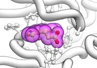 Example in which the current object is shown as ribbon with ligands in cpk and surrounding side chains as xsticks:
  GRAPHICS.sketchAccents = yes
  GRAPHICS.ribbonWorm = yes
  GRAPHICS.wormRadius = 1.
  GRAPHICS.quality = 20
  GRAPHICS.stickRadius = 0.25
  GRAPHICS.ballRatio = 1.1
  GRAPHICS.transparency[1] = 0.6
  GRAPHICS.hetatmZoom = 1.1
  color background white
  color residue label black  # if you decide to display them
  display ribbon white
  display a_H cpk magenta
  display a_H xstick
  display Res(Sphere( a_H a_!H,W//!c,ca,n,o,h*  )) & !a_*.//n,o,h* xstick white
  color xstick a_!H,W//n* lightblue
  color xstick a_!H,W//o* lightpink
#  display residue label a_//DX
GRAPHICS.hetatmZoom |
The default ball and stick radii of a ligand can be different by the GRAPHICS.hetatmZoom factor. This makes a better ligand view since the ligand stands out from the surrounding protein atoms.
See also, icm.clr file about changing the default color for carbon atoms in ligands (a.k.a. hetatm ) ( atom H color ) Default (1.5)
GRAPHICS.hydrogenDisplay |
determines the default hydrogen display mode for the display command.
 GRAPHICS.hydrogenDisplay = "polar"
        1 = "all"   # all hydrogens are shown
        2 = "polar" <-- current choice  # polar displayed, the non-polar hidden
        3 = "none"  # no hydrogens are displayed
GRAPHICS.light |
a rarray of 13 elements between 0. and 1. which controls the main properties of lighting model in GL. The sections of this array can be changed with four sliders of the Display tab in a top tool bar. The following elements are defined:
| Elements Property Range Default Comment |
|---|
| GRAPHICS.light[1] shininess 0.,1. 1. property of the solid material |
| GRAPHICS.light[2:4] ambient light 0.,1. {0.15 0.15 0.15} intensity of RGB for ambient light |
| GRAPHICS.light[5:7] diffuse light 0.,1. {0.6 0.6 0.6} intensity of RGB for diffuse light |
| GRAPHICS.light[8:10] specular light 0.,1. {0.35 0.35 0.35} intensity of RGB for specular light |
| GRAPHICS.light[11:13] emission 0.,1. {0. 0. 0.} intensity of RGB for emitted light |
To re-render the solid graphics with new parameters, use the
display new reflectioncommand.
Example:
build string "se his trp glu"
display cpk
color background blue
GRAPHICS.light[5:7] = {0.2 0.2 0.6}
display new reflection
See also: GRAPHICS.lightPosition .
GRAPHICS.lightPosition |
X,Y and Z posiion of the light source in the graphics window. The X and Y coordinates are usually slightly beyond the [-1. 1] range where [-1.,1.] is the size of the window, and the Z position is perpendicular to the screen and is set to 2. (do not make it negative). The default values are the following:
GRAPHICS.lightPosition = {-1.,-2.,2.}
See also: GRAPHICS.light .
GRAPHICS.mapLineWidth |
relative width of lines and dots of a displayed map . This parameter can be changed from the File/Preferences/DisplayGeneral menu.
See also: lineWidth , GRAPHICS.grobLineWidth , map , GRAPHICS.hbondWidth .
Default (1.)
GRAPHICS.occupancyDisplay |
preference controlling if and how the partial or zero atom occupancies are displayed. The abnormal occupancies are shown as circles around atoms. These following values are allowed.
- = "none" # nothing is displayed
- = "circle" # a circle is displayed
- = "label" # a circle and a label with the value (zero values are not shown)
A silly example.
GRAPHICS.occupancyDisplay="label"
build string "se ala his"
set occupancy a_//n* 0.5
display xstick
See also:
GRAPHICS.occupancyRadiusRatio |
The radio of a circle showing non-1. occupancy atoms to the van der Waals radius of the atom.
Default value: 1.5
See also:
GRAPHICS.quality |
integer parameter controlling quality (density of graphical elements) of such representations as cpk, ball, stick, ribbon . Do not make it larger than about 20 or smaller than 1. This parameter supersedes the previous ballQuality parameter.
We recommend to make this parameter at least 15 if you want to make a high quality image. You can also increase the number of image resolution by making the image window 2,3,4 times larger (in the example below it is 2 times larger) than the displayed window.
GRAPHICS.quality = 15
display ribbon

# press Ctrl-D  for the fog effect, move clipping planes, change fogStart

write image png window=2*View(window)
Default: 5.
GRAPHICS.rainbowBarStyle |
determines if and where the color bar will appear after a molecule is colored by an array. Coloring by an array is one of the options of the display and color commands.
- = "left" <- default choice
- = "right"
- = "no text"
- = "no bar"
GRAPHICS.resLabelDrag |
if yes, enables dragging of the displayed residue labels with the middle mouse button. The labels can be reset to their initial positions with the set residue label distance rs_
command. The initial position is defined by the relative displacements of {0. 0. 0.} from the special "residue label-carrying" atom of the residue, see the set label as_ command. See also resLabelStyle
Default ( no ).
GRAPHICS.resLabelYShift |
a non-negative integer number of spaces preceding a residue label that shifts it to the right (Y axis). This parameter is useful for displaying residue labels next to a solid representation, such as xstick , ribbon or cpk.
See also: GRAPHICS.atomLabelShift, GRAPHICS.resLabelDrag and s_labelHeader
Default ( no ).
GRAPHICS.ribbonCylinderRadius |
GRAPHICS.ribbonCylinderRadius is the real radius of helical cylinders in schematic protein topology display for the ribbonStyle = "cylinders" preference.
The radius can be set to zero for an automated, variable-radius mode or to a specific radius. Example:
read pdb "1crn"
ribbonStyle = "cylinders"
GRAPHICS.ribbonCylinderRadius = 2.2
display ribbon
See also:
GRAPHICS.ribbonGapDistance |
The minimal distance between the first atoms of the neighboring residues when the ribbon gap will be drawn if l_breakRibbon logical is set to yes. You can also control the display style of gaps with the GRAPHICS.chainBreakStyle variable.
Default: 4. See also: GRAPHICS.chainBreakStyle
GRAPHICS.ribbonRatio |
real ratio of depth to half-width for the protein ribbon .
Warning: note that this parameter influences
GRAPHICS.wormRadius if GRAPHICS.ribbonWorm is set no no .
In this case GRAPHICS.wormRadius will be redefined as GRAPHICS.ribbonWidth * GRAPHICS.ribbonRatio automatically.
Default: 0.3
See also: residue field "_WORMRADIUS_" for variable ribbon radius of the worm representation.
GRAPHICS.ribbonWidth |
real width of the protein ribbon .
Default: 1.
GRAPHICS.ribbonWorm |
logical parameter, if yes, makes the ribbon round, rather than rectangular.
See also: residue field "_WORMRADIUS_" for variable radius of the worm representation. Example:
read pdb "1crn"
GRAPHICS.ribbonWorm=yes
set field a_A/ Bfactor(a_/A )/3. name="_WORMRADIUS_"
display ribbon
Default: no
GRAPHICS.rocking |
preference with the following options:
- = "X-rocking"
- = "Y-rocking"
- = "Xy-rocking"
- = "xY-rocking" <-- current choice
- = "X-rotation"
- = "Y-rotation"
Default: 4
GRAPHICS.rockingRange |
real value of rocking range.
Default: 1.
GRAPHICS.rockingSpeed |
real value of rocking or rotation speed.
Default: 1.
GRAPHICS.selectionLevel |
preference for the selection level of as_graph selection. The atoms, residues, molecules or objects selected interactively in the graphics window are automatically stored in the as_graph variable. The preference may have the following values.
  GRAPHICS.selectionLevel = "atom"
        1 = "object"
        2 = "molecule"
        3 = "residue"
        4 = "atom" # default
        5 = "variable"
The GRAPHICS.selectionLevel can be switched either interactively, e.g.
GRAPHICS.selectionLevel = 3or from GUI by selecting the level combo box with the following choices: O (object), M (molecule), R (residue), x (atom), or an icon of a torsion (variable).
GRAPHICS.selectionStyle |
preference for the style in which the graphical selection is shown. The preference may have the following values.
  GRAPHICS.selectionStyle = "color"
        1 = "none"
        2 = "cross" # the default choice
        3 = "color"
        4 = "both"
In the 1-st mode ( "none") only a single selection mark is shown. It is convenient when
you do not want multiple selection marks to overwhelm the image.
The 3-rd mode is incovenient if you want to try different colored displays for the selected fragments.
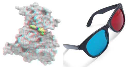
GRAPHICS.stereoMode |
- "up-and-down"
- "line interleaved" # current choice
- "in-a-window"
- "Sharp"
- "Anaglyph"
The "line interleaved" mode can be used with a new type of frame splitter at the line level. In this case the odd lines from one stereo-image are interleaved with the even lines of another. The side-effect of this mode is that the intensity is reduced in half since at each moment one sees only one half of the lines. The splitter device for this mode can be purchased from Virex (www.virex.com). This mode produces a dark stereo image but is easily available (requires stereo goggles, e.g. from Virex).
The "in-a-window" mode is used in SGI workstations and in a Linux workstation with an advanced graphics card supporting a quad graphics buffer. In this mode the hardware stereo regime applies only to an OpenGl window. This is the best mode but it requires an expensive graphics card (plus the stereo goggles).
Note: LCD screens can not display a stereo image since the image is not continuously updated at high frequency. This technical problem may be solved in the future (so we hear).
The "Sharp" option is for SHARP manufactured 3D screens.
The "Anaglyph" option is for the stereoscopic 3D effect achieved by means of encoding each eye's image using filters of different (usually chromatically opposite) colors, typically red and cyan. The Anaglyph option is the easiest to used with inexpensive 3D glasses and and without any expensive 3D compatible hardware or monitors.
GRAPHICS.stickRadius |
radius (in Angstroms) of a cylinder displayed as a part of stick or xstick graphical representation of a molecule.
Individual (residue-wide) control of stick radii.
In order to modify the default values of the radii from the command line use the set xstick r_newradius command For example:
set xstick a_/13:15 0.5In this case the ball radius will be changed according to the radio of the default parameters (e.g. GRAPHICS.ballRaduis/GRAPHICS.stickRadius )
Default (0.4).
GRAPHICS.surfaceDotSize |
Determines the size of the dot on the solvent accessible graphical surface area . This surface is controlled by the GRAPHICS.surfaceProbeRadius radius. If this parameter is changed, use
display surface refreshto update the dot size.
Default (2.0).
GRAPHICS.surfaceDotDensity |
Determines the number of dots per square Angstrom on the graphical solvent accessible surface area . Do not confuse this parameter with surfaceAccuracy . The latter controls the surface and energy calculation and does not affect the displayed surface.
See also: GRAPHICS.surfaceProbeRadius and GRAPHICS.surfaceDotSize. Default (10).
GRAPHICS.surfaceProbeRadius |
An increment to the van der Waals radii of atoms at thich the dotted atomic surface is calculated. It is used by the display surface command to display dotted van der Waals surface. If the GRAPHICS.surfaceProbeRadius is set to 1.4 the surface becomes equivalent to the solvent accessible surface with a probe of 1.4A (e.g. in show surface area ) .
Note, that in contrast to GRAPHICS.surfaceProbeRadius, the vwExpand parameter is used for calculations of the solved accessible areas (e.g. show surface area ).
Default (0.1)
GRAPHICS.transparency |
Two parameters regulating the transparency of grobs.
- GRAPHICS.transparency[1] contains a value from 0. to 1. representing the level of transparency (0. solid, 0.99 - invisible)
- GRAPHICS.transparency[2] contains the brightness of the transparent surface from 0. to 1.
GRAPHICS.wormRadius |
radius of coiled segments (i.e. those where the secondary structure is marked as "_") of a polypeptide chain in ribbon representation.
Warning: this parameter behaves as independent only in the GRAPHICS.ribbonWorm is yes . Otherwise, in case of a mixed ribbon representation display, ICM will reset the radius to the product of GRAPHICS.ribbonWidth and GRAPHICS.ribbonRatio in order to match thickness of the ribbon and the connecting coil. To make a variable worm radius of the cylinder set the residue field with a name "_WORMRADIUS_" Example:
read pdb "1crn"
GRAPHICS.ribbonWorm = yes
display ribbon  # uniform radius
set field a_A/ Bfactor(a_A/  )/3. name="_WORMRADIUS_"
display ribbon  # variable radius
Default (0.3).
GRID |
[ GRID.gcghExteriorPenalty | GRID.margin | GRID.maxEl | GRID.minEl | GRID.maxVw | GRID.gpGaussianRadius ]
parameters for the grid energy calculations (see also "gh,gc,ge,gs,sf" energy terms).GRID.gcghExteriorPenalty |
A preference to allow automatically impose a repulsive penalty outside the area covered by the van der Waals maps ( m_gc and m_gh ).
- = "repulsive" <- the default
- = "zero"
See also: gcMethod , GRID.margin
GRID.margin |
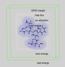
|
real parameter determining the extra penalty-free space around the map bounding box if GRID.gcghExteriorPenalty = "repulsive" (see above). For any atom which gets outside the map-bounding box expanded by GRID.margin, its grid van der Waals energy ( "gc" or "gh" ) is penalized by the GRID.maxVw value. This is the same penalty value which atoms get if they severely clash with other atoms. |
Therefore, if you set up grid energy calculations it is essential either to create a big enough box or set a sufficient margin to allow ligand rearrangements near the receptor surface. If GRID.margin is very large, your ligand will be "on the loose" and may spend too much time flying in open air. It is recommended that the margin is not larger than the diameter of your ligand.
Default: 0.00 A
See also: GRID.gcghExteriorPenalty , GRID.maxVw
GRID.maxEl |
real truncation parameter. Default: 20.0 kcal/mole.
GRID.minEl |
Default: -20.0 kcal/mole.
GRID.maxVw |
The truncation level of the van der Waals repulsion energy pre-calculated in the "gc" grid energy term. This number also is used as a penalty for the atoms outside the map box expanded by GRID.margin .
Default: 3.0 kcal/mole.
GRID.gpGaussianRadius |
The radius of the density Gaussian used to generate the property maps. Default: 1.2 A. See also:
- term "gp"
- set type property I_atomTypes R_upToSevenWeights
- make map potential "gp"
GROB |
[ GROB.atomSphereRadius | GROB.relArrowSize | GROB.arrowRadius | GROB.relArrowHead | GROB.contourSigmaIncrement ]
Parameters related to graphics objects. See also the Grob family of functions.GROB.atomSphereRadius |
default radius (in Angstroms) which is used to select a patch on the surface of a grob. Used in the color grob as_selection color command. See also: Grob( g R_6) function to return a patch of certain color.
Default: 4.0.
GROB.relArrowSize |
a real relative arrow size ([0.,1.]). Default: 0.2.
GROB.arrowRadius |
a real arrow radius in Angstroms used by the Grob( "ARROW", R_ ) function.
See also: makeAxisArrow , GROB.relArrowHead and GROB.`relArrowSize . Default: 0.5.
GROB.relArrowHead |
a real ratio of the arrow head radius to the arrow radius. This parameter is used by the Grob( "ARROW", R_ ) function. Default: 3.0.
GROB.contourSigmaIncrement |
a real increment in the sigma level used to re-contour an electron density map using the make grob m_eds add r_increment command.
This parameter is used in the GUI when plus and minus are pressed.
Default (0.1)
GUI |
[ GUI.autoSave | GUI.autoSaveInterval | GUI.defaultLayoutAction | GUI.displayNDValueStyle | GUI.tableRowMarkColors | GUI.windowLayout | GUI.workspaceStyle | GUI.workspaceTabStyle | GUI.workspaceFolderStyle ]
This parameter table contains some settings for the GUI (see below). Most of the settings are stored automatically in the s_userDir + "/config/icm.cfg" fileTo read about generating dialogs and menus from ICM see gui .
GUI.autoSave |
a logical to activate the saving of the content of the session every GUI.autoSaveInterval seconds. If the program exists unexpectedly or crashes the session then can be restored.
GUI.autoSaveInterval |
The number of seconds the session will save itself into a backup file as a precautionary measure against an unexpected termination or crash (see GUI.autoSave ) .
GUI.defaultLayoutAction |
The behavior of ICM windows upon clicking the "Default Layout" button (third at the left bottom corner). The "Main" location is the upper right window that gets maximized upon pressing the fourth button.
  GUI.defaultLayoutAction = "3D to Main"
        1 = "3D to Main" <-- current choice
        2 = "Tables to Main"
        3 = "Alignmnets to Main"
        4 = "Html To Main"
        5 = "Keep Main"
GUI.displayNDValueStyle |
The display of 'not-defined' values in rarray . Preference "empty" will leave the cell empty. The default will show letters ND .
  GUI.displayNDValueStyle = "text"
        1 = "text" <-- current choice
        2 = "empty"
Example:
GUI.displayNDValueStyle = "empty"
GUI.tableRowMarkColors |
E.g.
GUI.tableRowMarkColors = "#ff4444/#ffbb44/#44ff44/#4499ff/#ff44ff"
GUI.windowLayout |
defines one of the two alternative ICM-panel layout styles:
- = "traditional"
- = "widescreen"
GUI.workspaceStyle |
defines the look for objects and molecules in the ICM workspace panel.
- = "all"
- = "simple"
GUI.workspaceTabStyle |
allows one to change the style of ICM-object tabs created in the workspace panel of ICM GUI.
- = "icon title" # default
- = "icon"
- = "title"
GUI.workspaceFolderStyle |
defines how many hierarchical levels of 3D molecular objects are shown in the Workspace panel.
- = "closed"
- = "object"
- = "molecule" <-- current choice
- = "residue"
IMAGE |
[ IMAGE.quality | IMAGE.printerDPI | IMAGE.lineWidth | IMAGE.scale | IMAGE.stereoBase | IMAGE.stereoAngle | IMAGE.gammaCorrection | IMAGE.color | IMAGE.compress | IMAGE.generateAlpha | IMAGE.stereoText | IMAGE.previewer | IMAGE.previewResolution | IMAGE.lineWidth2D | IMAGE.bondLength2D | IMAGE.font | IMAGE.orientation | IMAGE.paperSize | IMAGE.rgb2bw | IMAGE.writeScale ]
table contains settings used by the following commands creating image files:IMAGE.quality |
this integer parameter allows one to improve quality of vectorized postscript images saved by the write postscript command. Actually this parameter only changes one number in the header of a postscript file. You can also manually edit the file to correct this number. This number defines the number of divisions of larger triangles into smaller ones accompanied by interpolation of colors which occurs during printer interpretation of the postscript stream to provide smooth continuous transitions. The optimal value of this parameter depends on the maximal triangle size. It may grow as large as 100 for a single triangle on a page. Typically for a molecular image with molecular surface IMAGE.quality=3 is sufficient.
Important. Do not set the parameter to values higher than 5 for the molecular image, your printer will die!
Default: 3
IMAGE.printerDPI |
this integer parameter the printer resolution in Dot Per Inch (DPI). Important for the write image postscript command.
Default: 300
IMAGE.lineWidth |
this real parameter specifies the default line width for the postscript lines. See also IMAGE.lineWidth2D
Default: 1.0
IMAGE.scale |
real variable. If non zero, controls the image scale with respect to the screen image size. The screen image resolution (or Dots-Per-Inch) is usually 72. Let's assume printer DPI to be 300 (see the IMAGE.printerDPI parameter). In this case IMAGE.scale=1. will make the printed image the same pixel size (which is about 4 times smaller) than the screen image. For pixel images saved by write image postscript command integer IMAGE.scale values ( 2., 3., 4. ) are preferable. That is what auto mode (IMAGE.scale=0.0) is trying to do. This consideration is NOT important for the vectorized postscript images created by the write postscript command.
Default: 0.0 (i.e. auto mode: maximum size fitting the page in given IMAGE.orientation)
IMAGE.stereoBase |
real variable to define the stereo base (separation between two stereo panels) in the write image postscript and write postscript command.
Default: 2.35 inches, (~ 60mm)
IMAGE.stereoAngle |
real variable to define stereo angle (relative rotation of two stereo images) in the write image postscript and write postscript command.
Default: 6.0 degrees.
IMAGE.gammaCorrection |
real variable to to lighten or darken the image by changing the gamma parameter. A gamma value that is greater than 1.0 will lighten the printed picture, while a gamma value that is less that 1.0 will darken it. You may adjust your gamma correction parameter for your printer with respect to your display and add this setting to the _startup
Default: 2.0
IMAGE.color |
logical to save color or black_and_white ('bw') images. You can override this parameter by using the explicit bw option in the write image command.
Default: yes
IMAGE.compress |
logical to toggle simple lossless compression, standard for .tif files. This compression is required to be implemented in all TIFF-reading programs.
Default: yes
IMAGE.generateAlpha |
logical to toggle generation of the alpha (opacity) channel
for the SGI rgb, tif and png image files to make the pixels
of the background color transparent.
Be careful. The alpha channel is set to 1. for every pixel in
your image which has the same color as the background.
Therefore there is a danger that the same
color will be accidentally used inside your image.
If you nevertheless want to generate the alpha-channel, use
a rare color your background (not black, but rather green, e.g.
rgb = {0.,0.976,0.} .
Default: yes
IMAGE.stereoText |
logical to make text labels for only one panel or both panels of the stereo diagram.
Default: yes
IMAGE.previewer |
a string parameter to specify the external filter which creates a rough binary (pixmap) postscript preview and adds it to the header of the ICM-generated high resolution bitmap or vectorized postscript files saved by the write image postscript, and write postscript , respectively . This preview information is compliant with EPSI (encapsulated Postscript interchange file format) and is useful to see a draft image instead of a empty rectangle upon inclusion of the postscript file into other drawing and imaging software like IRIS showcase.
Default: "gs -sDEVICE=pgmraw -q -dNOPAUSE -sOutputFile=- -r%d –– %s"
IMAGE.previewResolution |
integer resolution of the rough bitmap preview added to the vectorized postscript file in lines per inch. Recommendations:
- 10 - very rough ( 1/10th of an inch )
- 20 - a reasonable preview but no fine details
- 30 - a fine preview, do not increase it any higher since the file will become too large.
IMAGE.lineWidth2D |
the default integer thickness of bonds in chemical 2D drawing that is preserved upon the Copy Image command. This is useful for adjusting the table display and cutting and pasting from ICM to external documents.
See also: write image chemical , IMAGE.font
Default: 1.5 pixels
IMAGE.bondLength2D |
real length of a chemical bond (in inches) in chemical 2D drawings upon the Copy Image command. To make your molecule large, increase it. This is useful for cutting and pasting from ICM to external documents. Default (0.4 inches)
IMAGE.font |
This string defines the font used for elements in a chemical drawing.
Default ( "15px Arial" )
IMAGE.orientation |
preference to specify image orientation.
- = "portrait" <- default
- = "landscape"
- = "auto"
Default: "portrait"
IMAGE.paperSize |
preference to specify paper size.
- = "Letter (8.5x11")" <- default
- = "Legal (8.5x14")"
- = "11x17""
- = "A4 (210x297mm)"
- = "A3 (297x420mm)"
Default: "Letter (8.5x11")"
IMAGE.rgb2bw |
rarray of 6 elements defining translation of rgb colors into black and white ('bw') grades. The array is {RED_scale, GREEN_scale, BLUE_scale, RED_bias, GREEN_bias, BLUE_bias} and the default values are {0.3125, 0.5, 0.1875, 0., 0., 0.}.
IMAGE.writeScale |
an integer parameter used to increase the image resolution in the Quick Image Write tool (see a little camera on the top toolbar). This tool uses the
write image png window= N * View(window)command where N defines if the image is N-times bigger than the screen image. This parameter can be changed from File/Preferences/Image dialog.
LIBRARY |
[ LIBRARY.men | LIBRARY.res ]
table containing string paths of the icm parameter files, which are loaded by the read library [mmff] command. The library files will be taken from the s_icmhome directory if no explicit directory is provided. Extensions are automatically added. Defaults:
 LIBRARY.bbt="icm"  # bond bending types
 LIBRARY.bci="icm"  # mmff bond charge increments
 LIBRARY.bst="icm"  # bond stretching types
 LIBRARY.clr="icm"  # colors, gui controls
 LIBRARY.cmp="icm"  # amino-acid comparison matrix
 LIBRARY.cnt="icm"  # distant restraint types
 LIBRARY.cod="icm"  # atom codes
 LIBRARY.hbt="icm"  # hydrogen bonding types
 LIBRARY.hdt="icm"  # hydration types
 LIBRARY.lps="icm.lps"  # loop database, rebuilt with write model [append]
 LIBRARY.men="icm.gui"  # GUI commands. can be reloaded with 'read gui'
 LIBRARY.mmbbt= "mmff"  # mmff bond bending
 LIBRARY.mmbst= "mmff"  # mmff bond stretching
 LIBRARY.mmtot= "mmff"  # mmff torsions
 LIBRARY.mmvwt= "mmff"  # mmff van der Waals
 LIBRARY.rst="icm"  # variable restraint types
 LIBRARY.tor="icm"  # precomputed icmff torsion params
 LIBRARY.tot="icm"  # torsion types
 LIBRARY.vwt="icm"  # van der Waals types
 LIBRARY.res={"icm","usr"}
Example:
 LIBRARY.res=LIBRARY.res // "./benz.res" # just append
 LIBRARY.cod="./newCodes.cod"
 read library
LIBRARY.men |
LIBRARY.men defines a string with a filename to the file with the menus.
Two possibilities:
- define LIBRARY.men in the _startup file for the desired menus to be activated
- The menus can later be extended with the read gui filename command.
# open the $ICMHOME/_startup file and add this line
  LIBRARY.men = Getenv("HOME")+"/.icm/icm.gui"  # now the ICM GUI will invoke your file
LIBRARY.res |
a string array or file names of the residue libraries . File extensions can be omitted, e.g. LIBRARY.res={"icm","user","./lib/mylibrary"}
OBJECT |
Controls atom requisites which are written to a file in the write object command. Extensions are automatically added. Defaults:
 OBJECT.bfactor  =yes
 OBJECT.charge   =yes
 OBJECT.occupancy=yes
 OBJECT.site     =yes
 OBJECT.display  =no
 OBJECT.library  =no
 OBJECT.auto     =no
Example:
 OBJECT.auto = no
 OBJECT.display = yes
 read object "crn"
 display ribbon a_/1:40
 set plane 2
 display cpk a_/12
 write object "tm"  # graphics and planes are written
 delete a_*.
 read object "tm"
PLOT |
[ PLOT.box | PLOT.color | PLOT.font | PLOT.fontSize | PLOT.gridLineWidth | PLOT.lineWidth | PLOT.markSize | PLOT.numberOffset | PLOT.Yratio | PLOT.logo | PLOT.orientation | PLOT.seriesLabels | PLOT.labelFont | PLOT.rainbowStyle | SEQUENCE.restoreOrigNames ]
Contains settings used by the plot command. All real sizes are expressed in the Postscript "points" equal to 1/72" ( about 1/3 mm ).
PLOT.box |
rarray of the origin and relative sizes of the ICM plot frame: { X_origin, Y_origin, X_size, Y_size }. Box {0. 0. 1. 1.} fits the page optimally.
Default ({0. 0. 1. 1.}).
PLOT.color |
logical to generate a color plot. Usually it does not make sense to switch it off because your b/w printer will interpret the color postscript just fine anyway.
PLOT.font |
preference for the title/legend font. The font size can only be redefined by editing the *.eps file (search for the number before the scalefont string). Available choices:
- 1 = "Times-Bold"
- 2 = "Times-Roman" <- default choice
- 3 = "Helvetica"
- 4 = "Courier"
- 5 = "Symbol"
PLOT.fontSize |
real font size. Any reasonable number from 3. (1 mm, use a magnifying glass then) to 96.
Default (10.0).
PLOT.gridLineWidth |
real width of grid lines. Use a small number (e.g. 0.01 for thin grid lines). Default (0.2).
PLOT.lineWidth |
real line width for graphs (not the frame and tics)
Default (1.0).
PLOT.markSize |
real mark size in points. Allowed mark types: line, cross, square, triangle, diamond, circle, star, dstar, bar, dot, SQUARE, TRIANGLE, DIAMOND, CIRCLE, STAR, DSTAR, BAR. Uppercase words indicate filled marks.
Default (1.0).
PLOT.numberOffset |
integer offset for the X-coordinate with the number option. This option is used in a number of macros generating multi-section plots for amino-acid sequences.
Default (0).
PLOT.Yratio |
real aspect ratio of the ICM plot frame. Using link option of the plot command is equivalent to setting this variable to 1.0. If PLOT.Yratio is set to 0. , the ratio will be set automatically to fill out the available box optimally.
Default (0.8).
PLOT.logo |
logical switch for the ICM-logo on the plot.
Default ( yes ).
PLOT.orientation |
preference for the plot orientation. Currently inactive. Default ( yes ).
PLOT.seriesLabels |
preference to indicate position of a series/color legend inside the plot frame. You can provide individual names for each series in the optional string array argument of the plot command. (e.g. plot M_XY1Y2 {"Title","X","Y","Ser 1","Ser 2"}) Available choices:
- 1 = "none"
- 2 = "right" <- default choice
- 3 = "left"
- 4 = "top"
- 5 = "bottom"
PLOT.labelFont |
preference for the data point label font. You can also redefine the font size with the PLOT.fontSize variable. Available choices:
- 1 = "Times-Bold"
- 2 = "Times-Roman" <- default choice
- 3 = "Helvetica"
- 4 = "Courier"
- 5 = "Symbol"
PLOT.rainbowStyle |
preference defining the color spectrum used by the plot area command. This command lets you plot a function of 2 arguments and show the function value by color. By default the plot command uses the minimal and maximal values of the provided matrix. You can enforce the range with the color option. Available choices:
- 1 = "black/white"
- 2 = "blue/white/red" <- default choice
- 3 = "blue/rainbow/red"
Example:
 read matrix  # def.mat is the default one
 PLOT.rainbowStyle=1
 plot area def display   # grey-scale, automatic min and max
 PLOT.rainbowStyle=3
 plot area def color={-10.,0.} display  # enforce new range
 PLOT.rainbowStyle=2
 plot area def transparent={-2.,8.} display
# low values - blue, middle [-2.,8.] - invisible, large red
SEQUENCE.restoreOrigNames |
When sequences from GenBank are read in ICM, they get a comment (or description) line that describes their original complicated name. The description gets this : " Orig.name: "origSeqName. This name can be restored upon writing in various formats including write alignment fasta if this flag is set to yes . By default this logical variable is set to no . Example:
delete a,b,c
make sequence 3 10 # creates sequences a b c
set comment a "an experimental sequence Orig.name: expr "
align a b c  # creates aln
write aln fasta "tmp" # keeps a b c, default should be no, unless you redefined it
write aln fasta "tmp" SEQUENCE.restoreOrigNames=yes  # restores the names.
SITE |
[ SITE.appendStyle | SITE.defSelect | SITE.labelOffset | SITE.labelStyle | SITE.labelWrap | SITE.showSeqSkip | SITE.wrapComment ]
This table contains parameters and preferences used to display the sites, or important residues.SITE.appendStyle |
SITE.appendStyle =
- "none"
- "merge source"
Allows to extend the site description with the name of a new sequence, even if the text of the description if the same in the copy site command. For example, if there is a site in two different sequences, say A_PIG A_DUCK, but they are being transferred to a third sequence with two consecutive copy site commands, the resulting description may indicate something like that:
- FT 135 135 ACT_SITE active site Serine (from A_PIG), if the style is 1
- FT 135 135 ACT_SITE active site Serine (from A_PIG,A_DUCK), if the style is 2
See also:
SITE.defSelect |
string of significant site types (shown as one letter abbreviations) Sequence identity in the alignment positions which have one of those sites is additionally rewarded in the alignment score calculation.
Default: "ABFGLMstepm"
SITE.labelOffset |
(default 5. A) the real offset of the site label with respect to the residue label atom.
SITE.labelStyle |
the style preference of the displayed site information:
- "none"
- "symbol" # one letter symbol, see site .
- "comment"
- "full"
SITE.labelWrap |
0.5 (inactive)
SITE.showSeqSkip |
the string of the site types skipped in the show sequence (or alignment) commands.
SITE.wrapComment |
the integer length of the comment line. The longer lines will be automatically wrapped in the graphics view. Default: 30
TOOLS |
[ TOOLS.edsDir | TOOLS.membrane | TOOLS.minSphereCubeSize | TOOLS.pdbChargeNterm | TOOLS.pdbReadNmrModels | TOOLS.rebelPatchSize | TOOLS.smilesXyzSeparator | TOOLS.superimposeMaxIterations | TOOLS.superimposeMinAtomFraction | TOOLS.superimposeMaxDeviation | TOOLS.tsToleranceRadius | TOOLS.tsShape | TOOLS.tsWeight | TOOLS.writePdbRenameRes ]
parameters for some ICM tools. The TOOLS.superimpose.. parameters control
the superimpose minimize
TOOLS.edsDir |
A directory for the electron density map repository. If this path is empty (i.e. TOOLS.edsDir=="" ) the loaded maps from are cashed into s_userDir + "/data/eds/" directory
See loadEDS and loadEDSweb
TOOLS.membrane |
This real array contains the geometrical parameters defining shapes with lipids or water
for implicit solvation calculations. The array may contain multiple sections of 5 elements each.
Each atom is considered either buried by other explicit atoms of the objects or exposed.
Five types of environment are possible depending on the surfaceMethod and the "sf" term, with the first one (the 'membrane') being suitable for the membrane modeling
- "membrane" ( surfaceMethod=4;set term "sf", exposed atom solvation density in col3 or col7 )
- constant tension ( surfaceMethod=2; set term "sf"; surfaceTension=0.02 )
- water ( surfaceMethod=2;set term "sf", exposed atom solvation density in col3 of icm.hdt )
- apolar ( surfaceMethod=3;set term "sf", exposed atom solvation density in col4 icm.hdt )
- vacuum ( set term "sf" off )
If the surfaceMethod is defined as "membrane" and term "sf" is on, then each atom can be either in water environment or in lipid environment. The attribution is done according to the atom coordinates and a series of shapes coded by the TOOLS.membrane array.
Each shape is coded by 5 numbers in the TOOLS.membrane array. The following shapes with lipid-like environment can be introduced.
| Name | Type(e1) | e2 | e3 | e4 | e5 | Description | Examples |
|---|---|---|---|---|---|---|---|
| membrane | 1 | z_bott | z_top | z_bmargin | z_tmargin | Z-membrane with transitional layers | {1.,0.,30.,5.,5.} |
| z-chimney | 2 | x1 | y1 | x2 | y2 | infinite rectangular beam in Z direction | {2.,-5.,-5.,5.,5.} |
| z-cylinder | 3 | xct | yct | radius | 0. | infinite round cylinder in Z direction | {3.,7.,7.,15.,0.} |
| cube | 4 | xct | yct | zct | half-edge-length | cube with defined center and half-size | {4.,0.,0.,0.,10.} |
| sphere | 5 | xct | yct | zct | radius | sphere with defined center and radius | {5.,0.,0.,0.,10.} |
Each shape only defines the environment inside itself and is applied sequentially. To define water environment inside preceding lipid shape, use the negative type, e.g. {..lipid_shape.., -4.,0.,0.,0.,3.} for a water cube of half size 3.. Examples:
TOOLS.membrane = {1.,0.,30.,5.,5.} # one membrane from z=0 to z=30A with 5A transitional layers
TOOLS.membrane = {5.,0.,0.,0.,4.,  5.,10.,10.,10.,4.} # two lipid spheres at 0,0,0 and 10,10,10
TOOLS.membrane = {5.,0.,0.,0.,6., -5.,0.,0.,0.,3.}    # a spherical layer, two concentric spheres
Example:
TOOLS.membrane = {1.,0.,30.,5.,5.}
set terms only "vw,14,hb,el,to,ss,ts,sf"  # sf is on
build string IcmSequence( "EACARVAAACEAAARQ" "nh3+" "coo-" )
set a_/A String("H",Nof(a_/A))  # make a helix
translate a_ {0. 0. 0.}
display xstick
display box {0. 0. 0. 50. 50. 30.}  # purple box for visualization
display origin
connect  a_   # position it roughly in the membrane
set selftether a_/8/ca {0. 0. 20.}  # to prevent it from flying away
TOOLS.tsToleranceRadius = 15.
montecarlo v_//V  # rigid placement
#
montecarlo v_//V,xi*  # flexible placement
See also: icm.hdt , surfaceMethod = 4 , energy term "sf"
TOOLS.minSphereCubeSize ( default = 5.) |
This parameter adjusts the minimal size of a cube for fast scanning of interatomic pairs. These calculation may be necessary when pairs of atoms are processes during an energy calculation or in a Sphere function. If an odd atom or group of atoms is far away from the rest of the object (an unusual and undesired situation), an exceedingly large number of cubes between the groups need to be created. In this case the minimal size of an edge needs to be increased to deal with those sparse atoms. If you see a warning involving this parameter, have a look at the coordinates of your object and make sure that the atom positions are correct.
TOOLS.pdbChargeNterm |
TOOLS.pdbChargeNterm logical to automatically charge the N-terminal residue in read pdb command if it matches the first residue in construct sequence in _SEQRES_ field of a PDB file.
Example:
read pdb "1crn" TOOLS.pdbChargeNterm = yes
convertObject a_ yes no no no yes no yes ""
See also read pdb
TOOLS.pdbReadNmrModels |
TOOLS.pdbReadNmrModels = "first"
- = "first" : reads only one model from a multi-model (e.g. NMR) pdb file
- = "all" : reads all models from a multi-model (e.g. NMR) pdb file and creates a separate object for each of them
- = "all stack" : creates one object and loads all other models as a stored cartesian stack
This preference is set to "first" by default. Resetting it to "all"is equivalent to option all in read pdb . Setting the preference to 3 is equivalent to the read pdb all stack s_pdbMultiModelFile command. Example:
TOOLS.pdbReadNmrModels = "all"
read pdb "1dkc"  # all 10 models are read in as a_1dkc_1., .., a_1dkc_10.
read pdb "1dkc" TOOLS.pdbReadNmrModels=3 # one object with a built-in stack is created
TOOLS.rebelPatchSize |
Defines resolution of the electrostatic coloring. Smaller values will lead to slower calculation but better results. You may try a range from 0.3 for relatively small proteins to 2. for very large ones.
Default: 1.
TOOLS.smilesXyzSeparator |
ICM has an option to generate smiles with coordinates which is a much more compact (and one line only) replacement for an mol / .sdf file
TOOLS.superimposeMaxIterations |
The maximal number of iterative superpositions with gradually improved weights in the superimpose minimize procedure that optimizes the weighted rmsd to find the best superposition core. Do not afraid to set this number to a very large one since the procedure will exit earlier if the convergence is achieved.
Default: 10
TOOLS.superimposeMinAtomFraction |
The minimal fraction of equivalent atom pairs that will be superimposed with significant weights in the superimpose minimize procedure.
Default: 0.5
TOOLS.superimposeMaxDeviation |
Determines the maximal atom deviation for determining the core subset of atoms for which the unweighted RMSD is reported in r_2out in the superimpose minimize procedure. The unweighted rmsd for a subset must be lower than this parameter.
Default: 2.0
TOOLS.tsToleranceRadius |
radius around atoms where the deviations from the target are not penalized
Default: (0.)
See also: selftether , term ts , TOOLS.tsShape
TOOLS.tsShape and TOOLS.tsShapeData |
This preference and a rarray of parameters supports positional restraints for all non-virtual atoms of the current object. It can be used concurrently with atom-specific selftethers and does not need the set selftether as command. Some selftethers can have individual status "box" (see set selftether ), these atoms are controled by that status and not TOOLS.tsShape preference. The TOOLS.tsShape preference has the following values:
  1 = "none" <-- current choice
  2 = "sphere"  # also a spherical layer if two radii are specified
  3 = "box"
The TOOLS.tsShapeData real array contains the parameters needed for a shape restraint. Note that while TOOLS.tsShape preference can be specified as an inline argument of a minimize or montecarlo command, the array can not. Therefore the values need to be filled before you call the command, e.g.
TOOLS.tsShapeData = {20.}  # radius of the sphere
minimize "vw,ts" TOOLS.tsShape=2
sphere.For the sphere option the radii and the center x,y,z parameters can be specified.
TOOLS.tsShapeData = { [ minimal_radius ] max_radius [ x y z ] }
The radii can be provided in any order. The default radius is 20. and the center of the spherical restraint is the origin ( {0. 0. 0.}
Examples:
 TOOLS.tsShapeData = {10.} # keep atoms inside R=10
 TOOLS.tsShapeData = {10. 10.} # keep atoms on the surface of the sphere R=10
 TOOLS.tsShapeData = {10. 15.} # penalty free is the spherical layer between R=10 and 15
 TOOLS.tsShapeData = {10. 15. 3. 3. 3.} # layer between R=10 and 15 around  3.//3.//3. center
 TOOLS.tsShapeData = {10.}//Mean(Xyz(a_//!vt*)) # do not let molecule fly beyond 10A from where it is now
box.
TOOLS.tsShapeData = {xmin ,ymin ,zmin ,xmax ,ymax ,zmax }
These six parameters are compatible with the Box function. Example:
TOOLS.tsShapeData = Box( a_// 3. )
#
TOOLS.tsShapeData = 100.//100.//-1.//100.//100.//1.  # keep atoms in 1A layer around Z-plane
individual atoms in a boxNote that a box defined by TOOLS.tsShapeData (need six numbers) can also be used by individual atoms set to interact with a box with the following command:
set selftether "box" as_selIn this case TOOLS.tsShape is ignored (can be set to "none" )
See also: selftether , term ts
TOOLS.tsWeight |
Weight for a special terms "ts" that can be used in minimize to tether the atoms to its initial set of coordinates (see selftether ). To keep only some atoms self-tethered, use option selftether= as_selfTetheredAtoms of the minimize command. The convert command and set selftether set them.
Example:
  build string "lys"
  randomize v_//x*
  minimize "vw,to,ts"  selftether=a_//ca,c,n  TOOLS.tsWeight=10.
Default: (0.)
See also: term ts , selftether , TOOLS.tsShape.
TOOLS.writePdbRenameRes |
Defines translation rules for the internal ICM residue names in show pdb or write pdb commands. For example, names ra for adenosine, or cyss for the bonded cysteins, can be translated to other names during the pdb export into ade or cyx . The format is the following: icm_res_name , exported_pdb_res_name ; ... , e.g.
TOOLS.writePdbRenameRes = "cyss,cyx;his,hid" # will rename two residuesSee also: show pdb write pdb .
WEBLINK |
This table contains definitions of types of web links used in the web, show html, and write html commands. The table is read from "WEBLINK.tab" file from the $ICMHOME directory. Change this file for your own definitions. The weblink specification is used to extend the argument string substituted for %s (e.g. "IL2_HUMAN" element of the table array linked according to the type
SP %s "http://www.aaa?%s" will be transformed into the <a href="http://www.aaa?IL2_HUMAN">IL2_HUMAN</a> link. If %Ns specification is used, only N characters of the argument string will be retain in the link. For example,
PDB %s "http://www.pdb?%4s" and 1xyz_a15_25 (specifying chain and residue range) will be translated into
<a href="http://www.pdb?1xyz">1xyz</a>_a15_25 which in your browser will look like this:
"AUTO" is another type which can be used in the link S_ "TYPE" ... expression. In this case the DB type is automatically recognized according the database reference string pattern (see also WEBAUTOLINK). An example table:
#>T WEBLINK
#>-DB------DR--LINK-------
 PDB     %s  http://www3.ncbi.nlm.nih.gov/htbin-post/Entrez/query?db=s&form=6&uid=pdb|%4s|&Dopt=g
 NCBI    g%s http://www3.ncbi.nlm.nih.gov/htbin-post/Entrez/query?db=s&form=6&uid=%s&Dopt=g
 EMBL    %s  http://www3.ncbi.nlm.nih.gov/htbin-post/Entrez/query?db=s&form=6&uid=emb|%s|&Dopt=g
 SP      %s  http://www3.ncbi.nlm.nih.gov/htbin-post/Entrez/query?db=s&form=6&uid=sp||%s&Dopt=g
 SPA     %s  http://www3.ncbi.nlm.nih.gov/htbin-post/Entrez/query?db=s&form=6&uid=sp|%s|&Dopt=g
 PROSITE %s  http://saturn.med.nyu.edu/srs/srsc?[PROSITE-acc:%s]
 MED     %s  http://www3.ncbi.nlm.nih.gov/htbin-post/Entrez/query?db=m&form=6&uid=%s&dopt=r
Example:
 read table "seqcomp.tab"  #contains references to different databases
 web SR link SR.NA1 "PDB" SR.NA2 "AUTO"
WEBAUTOLINK |
This table contains definitions of web link string patterns for automatic recognition in the web, show html, and write html commands. The table is read from the "WEBLINK.tab" file in the $ICMHOME directory. Change the file for your own definitions. Recognition is not perfect because the patterns overlap.
Example:
 read table "seqcomp.tab"  #contains references to different databases
 web SR link SR.NA1 "AUTO" SR.NA2 "AUTO"
| Prev xrMethod | Home Up | Next Other |