[ Read and Split | Build 2D QSAR Model | About the Model | Model Weights | Save and Share Model ]
| 2D QSAR Tutorial |
How to Learn from a data set and make a model:
First load in a table of data on which you wish to perform the learn and predict functions. See the tables chapter for more information on ICM tables.
Split data into training and test sets
There are two ways to split your data into a training and test set:
1. Random split
Randomly assign rows to the training and test sets and specify the percentage for training.
Navigate to Tools -> Table -> Train Split and select the Random tab. Choose the training set percentage; the remaining rows become the test set.
2. Kennard-Stone split
The Kennard-Stone method builds a representative training set by selecting diverse points from the dataset. In Tools -> Table -> Train Split, choose the Kennard-Stone tab and pick one of these strategies:
-
Maximum dissimilarity
Starts by selecting the two most dissimilar points, then iteratively adds the point that is farthest from those already chosen. This produces a training set that spans the full range of descriptor or chemical space. -
Hierarchical
Uses hierarchical clustering to group similar items, then selects representative points from each cluster. This ensures coverage of all regions of the data and is helpful when the dataset contains natural groupings.
- Read in your data e.g. chemical spreadsheet (e.g. File/Open SDF or .csv). It is usually recommended to Convert the IC50 to pIC50 (-LogIC50)
- Select Tools/Table/Build Prediction Model (Learn) or use the Chemistry/Build Prediction Model option.
- Enter the name of table with which you want to perform the predictions. You may locate your table from the drop down arrow menu.
- Select the Column from which you wish to learn. Use the drop down arrow to select. NOTE If the table does not contain any numeric (integer or real) columns, there is nothing to predict, so the "Build Prediction Model - Learn" button will be disabled. For classification models ensure your training column contains integers (e.g., 1 = active, 0 = inactive). The "Learn" dialog will allow you to train a classifier using the selected descriptors.
- Enter a name for the learn model.
- Select which learning method you wish to use from the drop down menu (PLS, PCRegression, Nearest Neighbor Kernel Regression, Random Forest Regression, Bayesian Classifier, Random Forest Classifier).
- Select whether you would like ICM to estimate the number of latent variables or you can specify a range. Latent Variables (LVs). LVs are the new, combined variables PLS creates to maximize the correlation between structure and activity. You can either let the software automatically estimate the optimal number using cross-validation (which is usually the best approach) or you can define the range yourself. Choosing the ideal number of latent variables prevents underfitting or overfitting.
- Select No Free Term Constraint:f(0)=0 if you would the PLS method to find a constant and add it to the model.
Descriptors
- Select which columns (descriptors) of your table you wish to use to 'learn'. You can select just the mol column or all numerical columns.
- If you are using chemical descriptors select the fingerprint method want to use Linear or Extended Connectivity Fingerprints (ECFP)
- Select Binary if you want to use Binary fingerprints - do not check if you want to use counted.
- Minimal chain length the minimal length of the chain of atoms, enumerated in each compound, usually it is 1 which means that you will consider an atomic composition numbers as descriptors. The typing of atoms can be customized with the map argument. .
- Maximal chain length the maximal length of the chain atoms and bonds enumerated in each compound Usually it is 3 or 4. Larger values of this parameter will lead to a large number of possible combinations. To overcome that, either the typing needs to be simple (e.g. only sp2 and sp3 property, regardless of the atom number), or the data set needs to be really large.
- Length - this is the total number of bins in a final fingerprint. Typically the size (either explicit or automatically estimated) is in a hundreds to thousands range. We recommend to check the auto option.
Test
- Select the number of cross-validation groups you wish to use or selected rows can be used for cross validation. The number of iterations will impact the speed of the calculation. 5 is the default number of groups but 2 would be the least rigorous and selecting the 'Leave-1-out' would be the most rigorous calculation.
- Bootstrapping generates statistics (R2, RMSD) for a random prediction and you should aim for there to be a significant difference between the random R2 and the model R2.
- Click on the learn button and a model will be created and placed in the ICM Workspace panel (left hand side).
All models are then stored in the ICM workspace as shown below. A number of options are displayed in the right click menu.
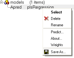
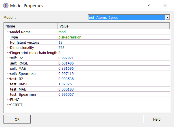
To see more details about your model (e.g. R2, RMSE etc....):
- Right click on your model in the ICM workspace and choose Model Data.
Predictive power is the primary measure of a model's performance and reflects its ability to generalize to unseen chemical space. External validation metrics quantify how well the model reproduces experimental trends and magnitudes for molecules excluded from training.
testR2 is the key indicator of external performance, representing the proportion of activity variance in the test set explained by the model. Values above 0.5 typically indicate robust generalization. testMAE measures the mean absolute deviation between predicted and experimental values for external compounds, providing an estimate of the model's average prediction error. testSpearman assesses the rank correlation of predicted versus experimental activities and is particularly informative when the model is intended for compound prioritization rather than precise potency prediction.
| Metric | Description |
|---|---|
| nofLatVec | Number of latent vectors used in the model (for example, PLS components). Each latent vector captures variance from descriptors relevant to activity. Too many can overfit; too few can underfit. |
| selfMAE | Mean absolute error on the training set. The average absolute difference between predicted and experimental values for molecules used to train the model. Measures how well the model fits known data. |
| selfR2 | Coefficient of determination on the training set. Fraction of activity variance explained within the training set. Higher means a better fit to known data. |
| selfRMSE | Root mean squared error on the training set. The square root of the average squared prediction error on training data. More sensitive to outliers than MAE. |
| selfSpearman | Spearman rank correlation on the training set. Measures how well the model preserves ranking order of activities. Useful when prioritizing compounds where order matters more than exact values. |
| testMAE | Mean absolute error on the external test set. The average error on molecules not used during training. Measures generalization to unseen data. |
| testR2 | Coefficient of determination on the test set. Fraction of activity variance explained on external data. A primary indicator of external predictive power. |
| testRMSE | Root mean squared error on the external test set. Similar to MAE but penalizes large deviations more. Useful to detect large outlier prediction errors. |
| testSpearman | Spearman rank correlation on the external test set. Measures ranking ability on unseen molecules. High values indicate the model can prioritize compounds effectively. |
The Weights dialog can be helpful to see what is driving the correlation in your model or for troubleshooting. The key column is "w" which represents the weight of the fragment in the regression. You may see a particular fragment providing a high weight to the model so you may want to add similar fragments to your training set to see if it will improve the model. Removing fragments from the training set based on their weight is not recommended because each fragment is part of a multiple component and it is difficult to know precisely its importance.
- Right click on the model in the ICM Workspace and choose Weights
- A table will be displayed containing the following columns:
name = smiles string of fragment. You can copy and paste this into the molecular editor to view it in 2D.
w = is actual weight of the fragment in the regression (used directly to get the result value).
mean = indicates the mean occurrence of the fragment in the model . For example, a value of 6 means the fragment is used 6 times in the regression.
rmsd = a high value indicates high occurrence of the fragment and influences the relative weight parameter.
wRel = relative 'importance' of the fragment based on the RMSD, mean and CorrY values.
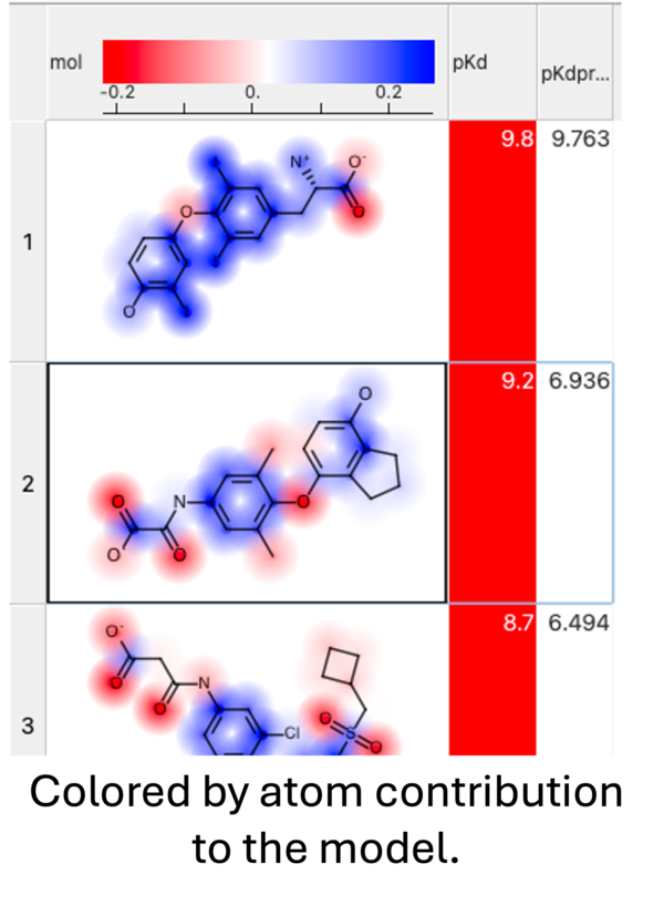
When you run the prediction you will see an option to color by atom contribution. This will color the atoms in the prediction results from negative (red) to positive (blue) based on their contribution weight (w column - see above) to the modek.
You can save and share a model by:
- Right click on the model in the ICM workspace (left hand panel) and choose Save As... This will save the model in MolSoft's .icb format.
- The .icb file can be opened in another session using File/Open