[ Molecule Representation and Color | Annotation | Labels | 2D and 3D Labels ]
Introduction
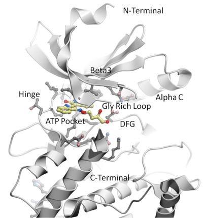
The following examples are focused on the structure of the kinase catalytic domain. The catalytic domain is nestled between the N- and C- terminal and has high sequence conservation between kinase families. The adenine moiety of ATP interacts with the hinge region which links the N- and C-terminals of the catalytic domain. The ATP sugar binding region is on the "floor" of the pocket where ribose makes a hydrogen bond with a polar residue. A conserved lysine residue on the beta3 strand is part of the "roof" of the pocket where the triphosphate group of ATP binds. A flexible glycine-rich loop moves in and out of the pocket depending on the ligand bound state of the PK and is regulated to some extent by the movement in and out of the pocket by the AlphaC helix. A buried region at the "back" of the pocket is protected by a "gatekeeper residue" forming a variable hydrophobic cavity. The hydrophobic cavity along with the DFG motif region are of interest for drug design because it opens up regions of the pocket which are not conserved and do not bind ATP.To learn the basics of the graphical user interface we will annotate the key structural regions of a protein kinase.
This tutorial shows you how to:
- How to load a PDB structure into ICM.
- How to change the background color.
- How to display and undisplay a molecule.
- How to color ribbon representation.
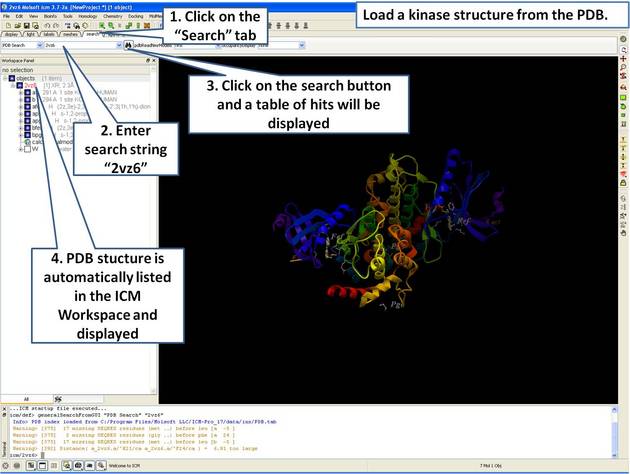 |
| Step 1: Click on the search tab to load and display the PDB structure 2vz6 |
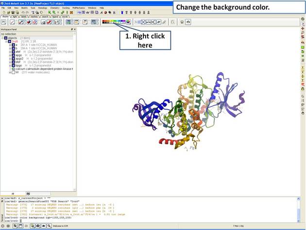 |
| Step 2: Change the background color by right clicking on the color palette. |
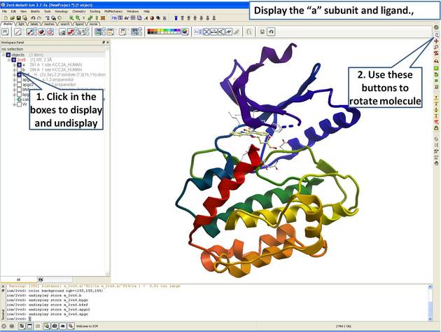 |
| Step 3: Display the "a" subunit of the kinase. |
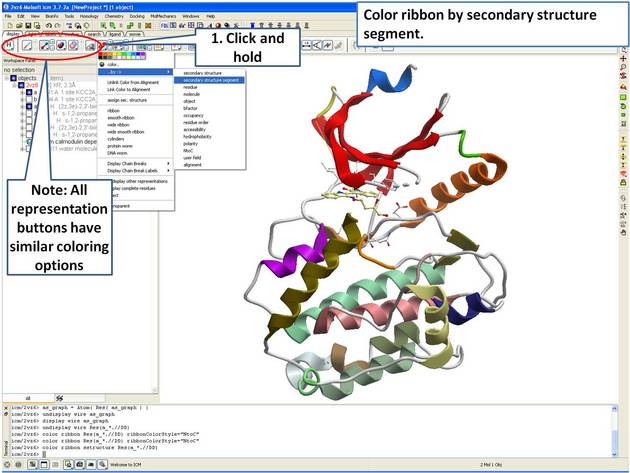 |
| Step 4: Use the options in the "Display Tab" to color the ribbon. |
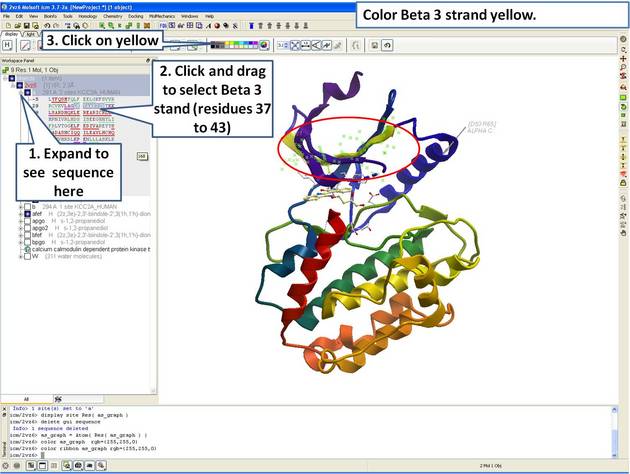 |
| Step 5: Select the beta 3 strand (residues 37:43) and color yellow. |
This tutorial shows you how to add user defined annotation to a particular region of a protein structure.
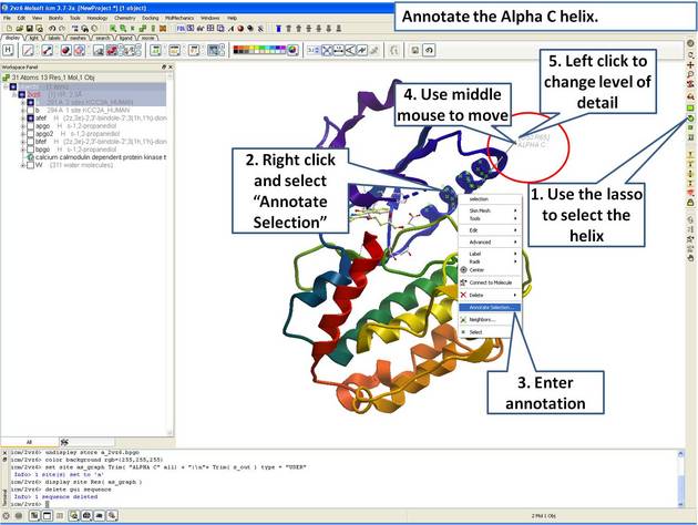 |
| Step 6: Select the region you wish to annotate and right click on the selection for options. |
This tutorial is a continuation from the previous tutorials in this section and shows you how to:
- How to select individual residue types.
- How to propagate a selection from one atom to all.
- How to use the residue label button.
- How to make a spherical selection.
- How to label a residue selection.
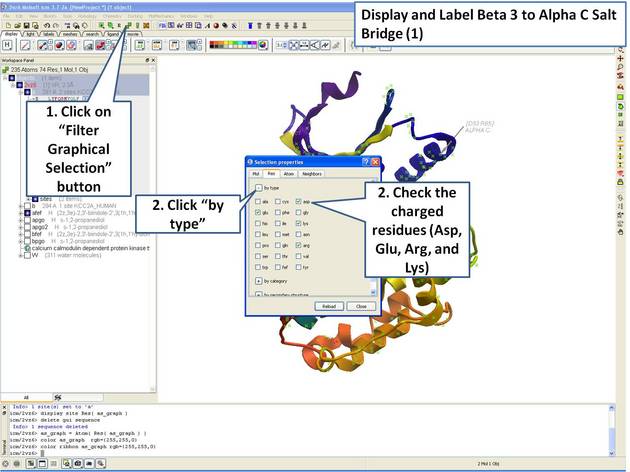 |
| Step 7: Use the "Filter Graphical Selection" button to select charged residues. |
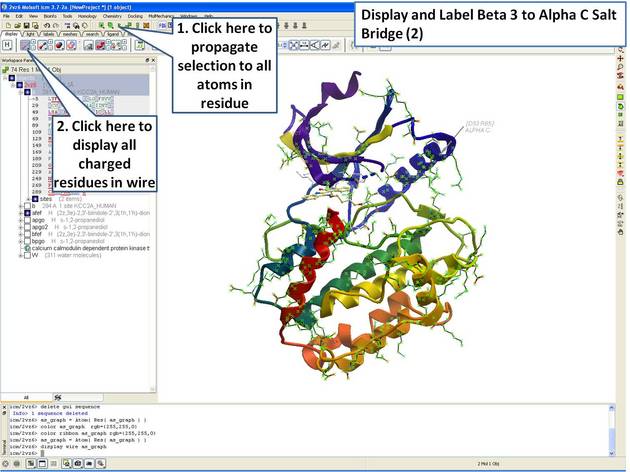 |
| Step 8: Propagate selection to all atoms to display all atoms of the side chain. |
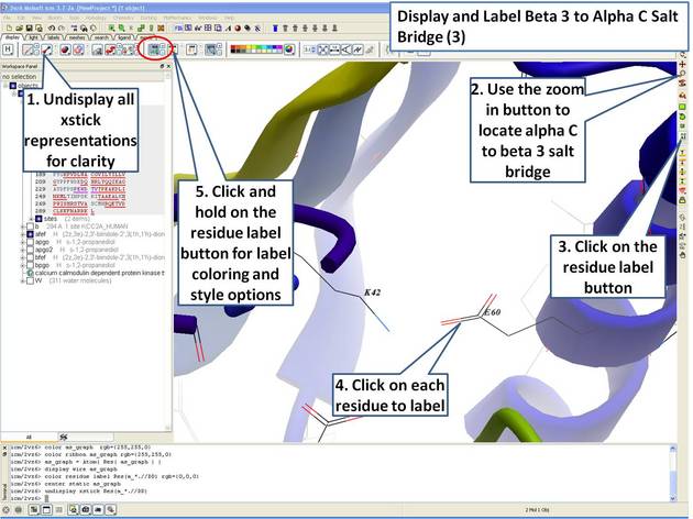 |
| Step 9: Locate the B3 to AlphaC salt bridge (K42- E60) and label using residue label button. Note: Once you have selected the two residues you can invert selection (click on invert selection button) and then undisplay all the other charged residues. |
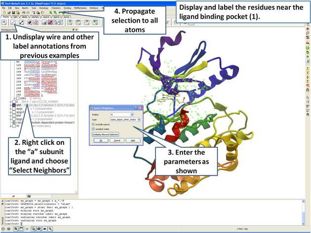 |
| Step 10: Select neighboring residues to the ligand. |
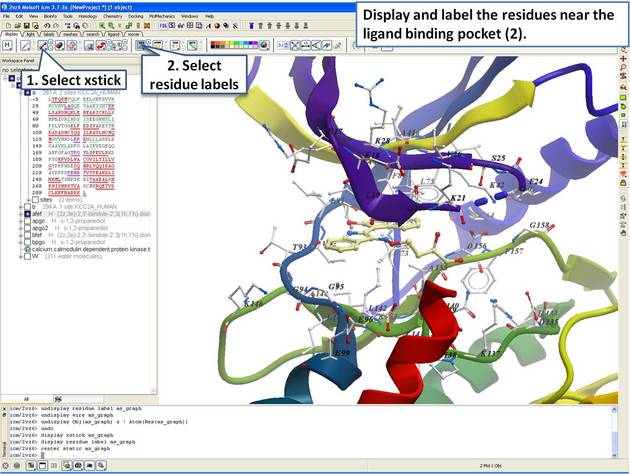 |
| Step 11: Display the residues and label them. |
This tutorial is a continuation from the previous tutorials in this section and shows you how to:
- Create and display a 2D label.
- Delete and move a 2D label.
- Create and display a 3D label.
- Delete and move a 3D label.
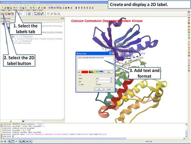 |
| Step 12: Create a 2D label using the options in the "labels" tab. |
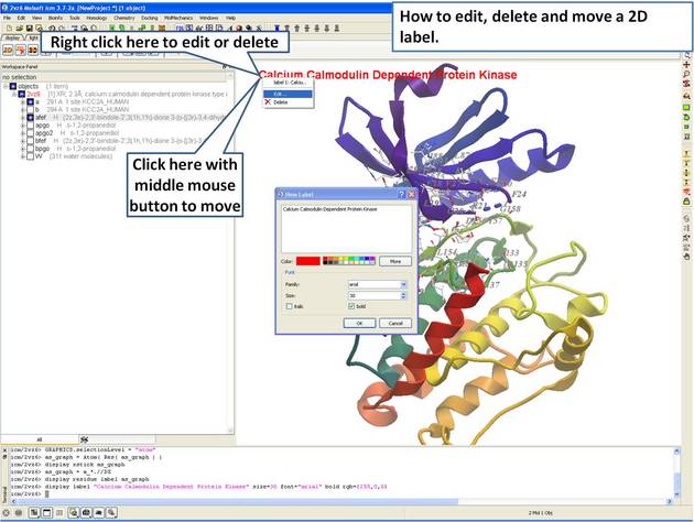 |
| Step 13: Right click on the 2D label to edit or delete it. |
 |
| Step 14: Create a 3D label using the options in the "labels" tab. |
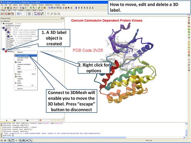 |
| Step 15: Right click on the 3D label to edit or delete it. |