Google Search the Manual:
Keyword Search:
| Prev | ICM User's Guide 17.5 Principal Component Analysis | Next |
| Available in the following product(s): ICM-Chemist | ICM-Chemist-Pro | ICM-VLS |
Principal Component Analysis (PCA) is the younger brother of ICM's more powerful data analysis tools, like property prediction and clustering, though it still may give a good description of the data with a few columns or even chemical compounds. PCA is a mathematical procedure that transforms a number of correlated variables into a number of smaller uncorrelated variables known as Principal Components The first component accounts for as much of the variability as possible with the rest of the components accounting for the remainder. PCA may be very helpful when you believe the data actually contains only a few meaningful components. Principal components are linear combinations of the provided data columns.
To perform a PCA analysis a table (either chemical or standard ICM table) needs to loaded into ICM. For information regarding ICM Tables and ICM Chemical Tables please follow these links.
To begin the PCA procedure
- Right click on a ICM Tables and ICM Chemical Table and select the PCA option. It is important to right click inside the data table and not on a column or row header in order to see the correct menu on which pca is listed.
- Select which columns you wish to incorporate into the PCA analysis.

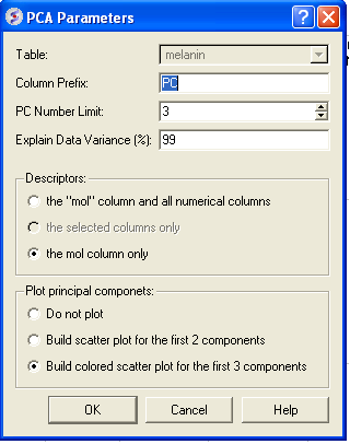
- Enter the table name on which you wish to perform the PCA analysis. If only one table is loaded this option will be greyed out.
- Enter the number of Principal Components (PC number limit) you wish to generate. Generally 3 principal components may be effectively visualized and it will be enough often to fulfil the data variance percentage requirement (see next option). The value displayed in the terminal window under the heading "cumulative explained data variance" will show what percentage of data relates to each PC.
- Enter a value in the "Explain Data Variance (%)" data entry box (99% is the default value) if you prefer this indirect way of limiting number of PC. The algorithm will stop when either PC number or explained variance limit is reached, so if you want only one of this criteria to work, make sure that the other limit is weak (by assigning accordingly the number of PC limit a high value, e.g. 50, or setting data variance to 100%).
- Select which descriptors you would like to include in the PCA analysis.
- Select which plot you would like to display. If you choose to display a plot use the color key on the side of the plot and the information contained within the ICM terminal window to relate which axes and points relates to which PC. PC3 is usually the color in the plot with the values displayed in the plot key.
- Click OK and if selected a plot will be displayed on the right-hand-side of the table. Points within a plot are linked to the table and can manipulated as other plots contained within a table.
| Prev Tooltips Balloons | Home Up | Next Learn and Predict |