[ Preference system | accessMethod | alignMethod | atomLabelStyle | atomSingleStyle | cnMethodAverage | compareMethod | dcMethod | electroMethod | errorAction | ExitSeslogStyle | ffMethod | gcMethod | highEnergyAction | interruptAction | mfMethod | minimizeMethod | pdbDirStyle | rejectAction | resLabelStyle | ribbonColorStyle | ribbonStyle | sequenceColorScheme | shineStyle | surfaceMethod | tzMethod | varLabelStyle | visitsAction | vwMethod | webEntrezOption | wireStyle | xrMethod ]
Preferences inside the shell are multiple choices (the outside persistent parameters are in ~/.config/Molsoft.conf , seepreference system ) .
You can show and list
them. This file can be just removed or moved to a different name to restore the original preferences. Also some known problems for older versions may be related to particular preference values.
You can change a preference by assigning it to:
- the item number
- the item name
- "nextItem" string
- 0 (the same as "nextItem")
Examples:
resLabelStyle = 3              # 3-rd choice
 resLabelStyle = "Ala 5"        # assign by string
 resLabelStyle = "nextItem"     # go to the next item in the list
Preferences are temporarily redefined just for one command , if specified
after the command, e.g.
minimize v_//x* electroMethod=2The ICM preferences can be divided into two groups:
- persistent, - the ones which user can modify and write with the
write system preferenceparName command. The location of the resulting file depends on the Operating System:- Unix: ~/.config/Molsoft.conf
- Mac: ~/Library/Preferences/com.molsoft.plist
- Windows: windows registry
GRAPHICS.chainBreakLabelDisplay - non-persistent: if you need to change them inside a script or in your
user_startupfile.
The persistent parameters can be found in the GUI menu under Preferences. The ones which are not on that menu, are non-persistent.
See also: preference system for the location of the file with modified user preferences and commands/ways to change them
The preferences can be divided into persistent and non-persistent as described above.
The non-persistent (like TOOLS.tsToleranceRadius ) need to be changed in a macro or script when needed.
The persistent ones can be searched and changed from the interface ( the File.Preferences menu ) or directly in a file between the ICM sessions for Unix and Mac.
From the command line one can change the preference and issue the write system preference prefName command.
User preferences in Linux.The user preferences (a subset of all preferences that can be modified in ICM)
can be modified by the user from the GUI (Menu File/Preferences).
The modified preferences are then stored in the
~/.config/Molsoft.conf file. You can modify those preferences manually provided there are no open ICM sessions.
Also, if you want to restore the defaults, simply delete the lines in question in Molsoft.conf.
User preferences on a Mac.The window size is stored in the ~/.icm/config/icm.cfg file. The rest of the preferences are in the Library/Preferences/com.molsoft.plist file.
open ~/Library/Preferences/com.molsoft.plist  # or
rm ~/Library/Preferences/com.molsoft.plistUser preferences on a Windows box:are stored in registry and can-not be easily viewed with a text editor (need registry viewer).
See also: write-system-preference command.
Defines if the show area surface command calculates absolute or relative
solvent accessible area for each atom. This area can be stored as absolute value in square Angstroms
or relative value from 0. to 1. and can be returned by the Area( as_ ) function.
Note that this preference does not work for residues. To calculate the relative residue area
use the Area( a_/* )/Area( a_/* type ) ratio of functions.
- "absolute surface" <-- current choice
- "relative surface"
- "multByAccMap"
show area surface a_1 a_1  accessMethod = 2 waterRadius=1.4
color a_1//* Area( a_1//* ) # returns numbers from 0. to 1.
The third method ("multByAccMap") uses m_ga map in a straightforward manner, just multiplies the atomic accessibilities by the map value. m_ga map is supposed to have values from 0. to 1.
Align and Score functions and
find database command (as described in Batalov and Abagyan, 1999).
- "ZEGA"
- "H-align" <- the best choice
- "frame-H-align" # align DNA sequence against protein sequence or protein sequence database
-
gapFunction, -
accFunction, -
alignMinCoverage(0.5) - minimal ratio of the aligned residues with respect to the shorter sequence length.
mmff
atom type.
Options are the following:
"cb1"<== default"cb1 q"(atomic charge)"cb1:FC"(formal charge and chirality)"cb1 all"(different atomic properties)"cb1 mmff q""C"(chemical atom name for non-H and non-C atoms, formal charge and chirality)"[C]"(chem. name, formal charge and chirality on a rectangle )"o,b"(occupancy,bfactor)"R/S"(R/S stereo labels, "R","S" or "")
Examples:
build string "se his"
 atomLabelStyle = "[C]"
 wireStyle = "chemistry"
 lineWidth = 3.
 display atom label wire black # press Ctrl-A
 color background white
 write postscript "tm"         # save the results
#
 atomLabelStyle = "C"
 display xstick
set type mmff # press Ctrl-A againwire mode.
- "tetrahedron"
- "cross"
- "dot"
GRAPHICS.ballRadius parameter and the line width
(especially important for the "dot" style) is controlled by the
lineWidth parameter.
method of calculating an effective distance for NOEs between groups of protons
This multi-center NOEs can be set with option all by this command:
set drestraint all as_group1 as_group2 i_TypeTwo methods are available for averaging.
cnMethodAverage  = "R6"
        1 = "R6" <-- current choice
2 = "nR6"r as r=(1/N Sum(r^-6))^-1/6, where N is n1*n2.The second mode calculates effective distance as r=(Sum(r-6))^-1/6
Depending on the number of protons in each group, the difference in the effective
distance may differ from 12 to 34%.
This method is usually set by the compare command. The last two methods
perform chemical equivalency matching.
compareMethod    = "variables"
        1 = "variables" <-- current choice
        2 = "atoms static"
        3 = "atoms superimposed"
        4 = "atoms interface"
        5 = "chemical static"
6 = "chemical superimposed"compare a_LIG.
compareMethod = 5
montecarlo
-
"exact"<- default -
"unnormalized"
- The
"exact"density correlation penalty function uses the Pearson's correlation coefficient. The correlation coefficient is then shifted by +1 so that the function ranges from0.to2.rather than from1.to-1.DC = 1 - Sum( Di - < D > )( Ai - < A > )/( N * Rmsd( D )*Rmsd( A )) The term has analytical derivatives with respect to the internal coordinates and can be efficiently locallyminimized. This term requires additional memory allocation equal to the current map size and is two times slower than the unnormalized term. - The "unnormalized" density correlation.
Formula:
DC = 1 - Sum( Di - < D > )( Ai - < A > )/ N
where Di is a map value in point i , and Ai represents the density generated
dynamically from atomic positions.
The differences from the
"exact"term are the following:- scaling is arbitrary in contrast to
"exact"term. Therefore you have to estimate a reasonabledcWeightvalue if"dc"is optimized along with the other energy or penalty terms. - The
"unnormalized"term does not require additional memory and is two times faster than the"exact"term. The term has analytical derivatives with respect to the internal coordinates and can be efficiently locally minimized.
- scaling is arbitrary in contrast to
- "Coulomb"
- "distance dependent" <- default
- "MIMEL"
- "boundary element"
- "generalized Born"
-
The Coulomb electrostatics is defined as U = q1 *q2 /D*r12
with D =
dielConst. -
In the distance-dependent dielectric model D in the above formula is set to
dielConst*r, whereris an interatomic distance. -
The "MIMEL" electrostatics allows one to evaluate the
free energy of a molecule in water environment by the
Modified IMage ELectrostatics
approximation at every iteration of the Monte Carlo, or
search procedure.
This energy will only be calculated for a static structure or
at the end of local minimization
( so called "double energy scheme", see
Abagyan and Totrov, 1994section (e) on p.992, orAbagyan, Totrov and Kuznetsov, 1994p. 10, for reference). ). The MIMEL energy consists of the Coulomb energy, which is calculated for all the atom pairs at the currentdielConstvalue, and the electrostatic solvation energy which is a sum of "selfEnergy" and "crossEnergy" and is returned in ther_outreal variable upon completion of the calculation in the show energy command. A more accurate evaluation of the electrostatic solvation energy can be obtained with theboundary elementmethod. -
The
boundary elementmethod provides an accurate solution of the Poisson equation. The dielectric boundary is defined by the accurateanalytical molecular surface(skin) and all the local charges stay exactly where they are. The boundary element method does not rely on any 3D grid and is free from dependence on the grid size. The ICM implementation of the boundary element method is fast and accurate. During the local minimization the derivatives with respect to the internal coordinates are not calculated (similar to the MIMEL method). The distance dependent dielectric model is used during minimization instead. At the end of the local minimization the electrostatic energy is replaced by the more rigorousboundary elementenergy. -
the generalized Born method is a faster method than
rebelthat relies on shape-derived estimations of the Born radii of charges the generalizerd Born approximation of the electrostatic energy. The implementation used here is desribed by Max Totrov in J Comput Chem. 2004 Mar;25(4):609-19. Good parameters for this method are the following: surfaceAccuracy = 5; make born; vwCutoff = 15; show energy "el" V_*;
- =
"none"# error flag is set (see the Error() function) - =
"break"<- default # exit from loops and macros - =
"exit"# exit from a script into shell - =
"quit"# quit ICM: useful for CGIs
Specific error messages can be suppressed with the
s_skipMessages ( e.g.
s_skipMessages = "[696][2073]" )
See also:
s_errorFormat,
interruptAction
Together with s_logDir controls where and what session files are saved upon exit/quit from ICM.
exitSeslogStyle = "full seslog" by default.
- = "none" # no files are saved
- = "full seslog" <-- current choice # all the macros and all the commands saved to seslog.icm
- = "user session" # only user commands saved to session.icm
- = "both" # both files are saved
minimize, and
montecarlo commands.
- = "ecepp" <- default
- = "mmff"
- = "icff" an experimental force field obtained by re-parametrization of the mmff force field into the internal coordinate space and derivation of the parameters specific for a particular covalent geometry.
- = "icmff" a new forcefiled (Arnautova,Abagyan,Totrov, Development of a new physics-based internal coordinate mechanics force field and its application to protein loop modeling. Proteins. 2011 Feb;79(2):477-98.). To activate it run the set_icmffmacro.
<> Note that minimize cartesian temporarily enforces ffMethod = "mmff", since the ecepp force field is not applicable to the cartesian minimization.
To use the force fields you need to do the following:
- "ecepp"
-
read library(if it is not included in your _startup.icm file) - modify terms with the
set termscommand. - use
show energy,minimize, ormontecarlo.
-
- "mmff" in cartesian space (free covalent geometry). The command requires
at least the
"vw,af,bb,bs" terms and needs correct atom types and charges.-
read library mmff - assign atom types:
set type mmff a_. This operation requires correct
-
- chemical structure (when you build the molecule, make sure it is complete),
-
bond types (check graphically with wireMethod=2, and change with the
set bond typecommand), and -
formal charges (check graphically with the
atomLabelStyle=3, and assign with theset charge formal ..command).- assign charges:
set charge mmff a_ - modify terms with the
set termscommand. The full set is:set terms "vw,el,to,af,bb,bs" - use
show energy,minimize, ormontecarlo.
- assign charges:
- "mmff" in the internal coordinate space according to the current fixation. The use of the mmff force field is not recommended.
- "icmff". This new force field is designed to be used with the fixed covalent geometry and is faster than both mmff-cartesian and "ecepp". The icmff force field is still experimental and should be used with caution. The vacuum part of icmff requires only three terms: "vw,to,el". The solvation terms "sf,en" can be added. Icmff calculates parameters on the fly for a particular geometry. To use this force field use the following procedures:
- assign mmff types and charges, and load the mmff libraries (see above)
- to generate the starting conformation, minimize your molecule
with
ffMethod = 2andminimize cartesian "14,to,bb,bs,af". - set ffMethod to 3 and
set terms ""vw,to,el,sf,en" only. - use show energy or montecarlo
m_gc map is used in the "gc" grid energy calculation.
The "gc" method allows one to calculate interactions of a molecule with grid energy field
representing another molecule ( the first method ), or treat the m_gc map as the electron
density map. To see individual atomic contribution, use show energy atom command which places individual energies in the bfactor field with a 20 unit offset.
"vw"<- default choice: current object interacts with the van der Waals field. Positive values repel, negative attract; Contribution from one non-hydrogen atom isEatom = 1.*Egc"density": treats them_gcmap as positive electron density and pulls the object into it. The contributions of atoms are proportional to atomic number (the number of electrons), hydrogens are ignored:Eatom = -AtomicNumber*Egc"field": uses user-defined atomicfieldvalue, which can be set by the set field command and extracted with theField(as_ ) command, as the relative weight of each atom. Anticipates that van der Waals type of the map (attractive negative values, repulsive positive) as in the first method.Eatom = Field(atom)*Egc
See also : GRID.gcghExteriorPenalty , GRID.maxVw , map
montecarlo
steps resulting in
no modification of a stack mnhighEnergy ,
(it means that conformations are dissimilar
to those in the stack and have higher energy).
Four actions can be taken:
- "heat"
- "stack-jump" <- default
- "random"
- "exit"
- =
"break loop" - =
"break all loops"<- default - =
"exit macro" - =
"exit to the main macro" - =
"exit all macros"
montecarlo, or minimize commands.
Allowed values:
-
"intermolecular"(or1) <- default -
"all"(or2)
mfMethod = 2 )
In contrast to the "vw" term, only intermolecular atom pairs are considered by default, since usually intramolecular interactions are calculated with the standard energy terms.
In the
"all" mode the atom pairs are taken from the van der Waals
interaction lists calculated dynamically in
the show energy, montecarlo, or minimize commands.
All atom pairs except atoms separated
by 1 or 2 bonds (so called 1-2 and 1-3 interactions) and within the vwCutoff
distance are taken into account.
See also: term "mf",
pmf-file, mfWeight .
minimize command, and is a part of one step of a multistep procedure
such as montecarlo, ssearch, and convert .
Allowed values:
-
"conjugate" -
"newton" -
"auto"<- default
"conjugate" means conjugate gradient minimization. Uses
analytical first derivatives and takes 6* n_free_variables memory.
"newton" - quasi-Newton method. It uses analytical
first derivatives and takes n_free_variables*n_free_variables
memory. We recommend this method for energy minimization of small molecules.
"auto" <- default; use the more efficient quasi-Newton
if the number of free variables (Nof(v_//*) is less than 100
(additional memory requirement of about 2 MB) and switch to
the conjugate gradient method if the number of free variables is more than 100.
s_pdbDir variable is set correctly, it is
sufficient to refer to the file by its four-character code, e.g.
read pdb
"1abc"
- "1abc.pdb"
- "pdb1abc.ent" <-- current choice
- "ab/pdb1abc.ent"
- "ab/pdb1abc.ent.Z"
- "ab/pdb1abc.ent.gz"
- "PDB website"
_startup file.
mnreject
trial conformations in a row. Four actions can be taken:
- "
heat" <- default choice - "
stack jump" - "
random" - " exit"
-
"A5"<- default choice -
"Ala 5" -
"ALA 5" -
"Ala" -
"ALA" -
"Alanine 5" -
"5" -
"A" -
" A" -
"Mol"- displays MOLECULAR name.
resLabelShift (Z-shift of labels on CPK and skin), atomLabelStyle .
| 1 = "type" | default. colors by secondary structure type or explicit color |
| 2 = "NtoC" | colors each chain gradually blue-to-red from N- to C- (or from 5' to 3' for DNA) |
| 3 = "alignment" | if there is an alignment linked to a protein, color gapped backbone regions gray |
| 4 = "reliability" | 3D Gaussian averaging with selectSphereRadius of alignment strength in space
|
ribbonColorStyle equals to 4, the conserved areas will be colored blue, while the most divergent
will be red, and the intermediate conservation areas will be colored white.
Example:
nice "1eoc.a/"
 make sequence a_1.1
 read pdb sequence "3pcc.a/"
 aa = Align(3pcc_a 1eoc_a)
 ribbonColorStyle=3   # color gaps gray
 color ribbon
 ribbonColorStyle=4   # see alignment strength
 color ribbon
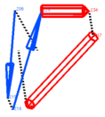
|
specifies type of representation when display ribbon command is used. Options are the following:
|
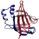
|
ribbon representation.
cylindersThe second representation draws alpha-helices as cylinders. There are two modes depending on the value of the
GRAPHICS.ribbonCylinderRadius parameter.
If GRAPHICS.ribbonCylinderRadius is set to zero, the automated radii fitting and helical splitting is engaged.
If a helix is too curved, ICM tries to split it into more straight helices.
The radius of a helix depends on the helical curvature and is calculated to include
all C atoms. Therefore, wide cylinders contain more curved helices.
Alternatively if GRAPHICS.ribbonCylinderRadius has a certain non-zero value, this radius will be used.
One can break a helix in any place with the assign sstructure command.
(e.g. assign sstructure a_/182 "_" to break a helix by residue 182 ).
The third and the fourth, "pencils" and "number" refers to a style where secondary
structure elements are represented by vectors (see
Abagyan and Maiorov, 1988).
Note The segment parameters must be pre-calculated with the
assign sstructure segment
command.
The last option ("both")
will display both representations of the backbone topology.
See also: GRAPHICS.chainBreakStyle (visibility of missing backbone segments).
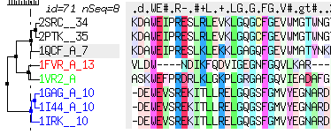
"no color""residue type""icm-combo" <-- current choice"consensus strength""greyscale"
CONSENSUS_strength parameter.
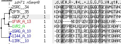
The last three preferences are illustrated below.
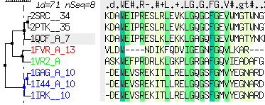
cpk , skin and grobs reflect light.
Possibilities:
"white"<- default"color"
"constant tension""atomic solvation"<- default choice"apolar""membrane"
"constant tension"means that the energy terms are just the product of the totalsolvent-accessible surfaceby thesurfaceTensionparameter. This term is intended to represent the surface energy if electrostatics takes the solvent polarization energy into account (seeelectroMethod)"atomic solvation"option is designed to evaluate the solvation energy purely on the basis of the atomic accessible surfaces instead of using the proper electrostatic evaluation of the polarization free energy. This fast but approximate scheme was proposed byWesson and Eisenberg, (1992). Atomic surface parameters derived from the experimental vacuum-water transfer energies are given in theicm.hdtfile."apolar"option is designed to evaluate the stabilization energy, which is the difference between denatured and folded states. The "atomic solvation" energy should be used with the van der Waals term while the "apolar" energy takes it into account and should be used without any other energy terms. The "apolar" atomic surface parameters were derived from the experimental octanol-water transfer energies and are given in theicm.hdtfile."membrane"option allows one to have a heterogeneous environment with shapes that are 'membrane-like' and shapes with water. The geometrical parameters and shape types are defined by theTOOLS.membranereal array. Depending on where an atom is found inside or outside the lipid shape the implicit solvation parameters will be taken from the 7rd column or the 3rd column of theicm.hdtfile.
m_ga grid map for correct calculations of the
surface accessibilities.
The method used to correct the accessibility values by the m_ga map can be modified with the accessMethod preference. If accessMethod = 3 , the atom accessibilities are multiplied by the m_ga value in the vicinity of the atom.
See also:
"simple": equal weight tethers to 3D points"weighted": individual weights are calculated from atomic B-factors by dividing8*PI2by the B-factor value. All the weights additionally are multiplied by thetzWeightshell variable."z_only": tethers are imposed only in the Z-direction towards the target Z-coordinate. These type of tethers pulls a molecule into a z-plane. This may be useful if you are trying to generate a flat projection of a three-dimensional molecule."function": tethers can take a form of distance restraints with individual weights, upper and lower bounds. The three parameters are controlled by the following properties of the target atoms (not the source atoms as in the"weighted"case): individual weights are directly taked frombfactorvalues, the upper bounds from theareafields, and the lower bounds from thechargefield. To set those values, use the set bfactor, set area and set charge commands respectively. Example:
applying linear force to atoms: to exert a constant force to an atom, set the formal charge of the target atom to a special value of 5. The b-factors will continue to serve as individual force constants and the direction of force will correspond to the vector from the origin to the target pdb-atom with this special value of formal charge.build string "se ala" copy a_ tether "tz" a_//T # movable source atoms a_//Z # static destination atoms Select(a_ "tz") # also, the destination atoms set bfactor a_tz.//* 3. # weight of each tether set area a_tz.//* 2. # no penalty within 2A radius around each atom set charge a_tz.//* 0. # the lower bound of 0. (can also create repulsion).
Example for the
"z_only" method in which we generate a more or less
flat image of a chemical.
build smiles "c1c(ccc(c1)N(=O)=O)N2CCC(CC2)=CC(=O)NNC(=O)Nc3cc(ccc3)C(F)(F)F"
tzMethod = "z_only"
set tether a_   # sets tethers to x,y,z=0. coordinates for each atom
minimize "vw,tz" 200
dsChem a_//!h*

#linear force. Use interface to set the linear force flag (formal charge) and bfactors
copy a_ "tzcopy"
tzMethod = "function" # will use bfactor and formal charge features of a_tzcopy. atoms
set tether a_/1/ca a_tzcopy./1/ca  # drag the target atom where you want
set charge formal a_tzcopy./1/ca 5. # number 5. signals ICM to interpret it as linear force
set bfactor a_tzcopy./1/ca 5000.    # the force constant
set tether a_/1/cb a_tzcopy./1/cb   # combine with normal tethers.
display tether a_
minimize v_//?vt* "tz"-
"greek"<- default choice -
"name" -
"value" -
"energy": value, torsion energy, and its maximal amplitude -
"ringsonly" -
"valueonly"
[ heat | stack-jump | random | mc-exit ]
what to do, if onestack
conformation is overvisited, i.e.
mnvisits
has been reached. The following actions are allowed:
-
"random" -
"heat"<- default choice -
"stackjump" -
"cross" -
"exit"
Explanation of actions:
-
"heat"- double the simulation temperature -
"stackjump"- jump to the conformation of the least visited slot in the stack. -
"random"- randomize all free variables according to themcJumpparameter -
"exit"- exit the MC procedure
van der Waals term ("vw").
The following three functions can be chosen:
"exact"<- default choice: Fvw = A/r12 - B/r6 . This is the usual van der Waals formula tending to infinity at r close to 0."soft":Fsoft = Fvw , for Fvw <= 0. and Fsoft = Fvw *(t/(t+Fvw )) for Fvw > 0. (repulsion). This form preserves the function for the most populated part of the curve but smoothly reaches the limitt(defined by thevwSoftMaxEnergyreal system variable)- "old soft": another smooth approximation with the finite value at r=0, depending on the well depth.
- "none"
- "g:GenPept" <- default
- "r:Report"
- "f:FASTA"
- "a:ASN.1"
- "d:Entrez document summary"
- "m:MEDLINE links"
- "p:protein neighbors"
- "n:nucleotide links"
- "t:structure links"
- "c:genome links"
See also:
s_webEntrezLink,
web,
show html,
write html.
- "wire" <- default choice
- "chemistry"
- "tree"
display virtual command.
Note: The "tree" graph does not exist for objects of non-ICM type, e.g. those created by the read pdb command, and this preference will have no effect. The tree representation elucidates the ICM topology graph imposed on molecules and is crucial in the
modify
command, since it removes a branch up-tree from the specified entry atom, and replaces
it by another branch. Use Ctrl-W to toggle between these styles (see set key command).
The line width is controlled by the lineWidth parameter.
- "corr Fc:Fo" <- default
- "corr Fc2:Fo2"