[ FFT Protein-Protein Docking | Protein-Protein Interface prediction | Setup | P-P Set Project | P-P Receptor Setup | P-P Ligand Setup | Epitope | P-P Maps | P-P Batch | Results | Refinement ]

Available in the following product(s): ICM-Pro

12.7.1 FFT Protein-Protein Docking

The Fast Fourier Transform (FFT) docking method contains two stages:

1. The first stage uses a simplified scoring function representing steric fit and hydrophobic/hydrophilic contact matching. FFT is then used for translational search using systematic search of rotations from 60x27 (coarse) to 256x125 (fine) orientations.
2. The second stage rescores the top 3000-20000 solutions with a more accurate energy function including electrostatics and SAS-based solvation. The conformations are then clustered using contact fingerprints.

Selected complexes in the stack of hits can then be refined with flexible side-chains.

See the tutorial here. Read the publication describing the method here.

12.7.2 Determination of Protein-Protein Docking Interface

The ICM Optimal Docking Area method is a useful way of predicting likely protein-protein interaction interfaces. If you do not have mutational data or other experimental data which indicates the likely protein-protein docking site this method will be useful. This procedure can save you time during the docking procedure by focusing your docking only on areas on the receptor and ligand most likely to interact.

12.7.3 Protein-Protein Docking Legacy Protocol

Here we describe the steps for protein-protein docking using the Legacy protocol. This method was superseded in 2015 by the FFT method. In this example we re-dock a complex of subtilisin and chymotrypsin (PDB code:2sni). The example will re-dock the ligand ( PDB code entry 2ci2) into the receptor molecule (PDB code 2st1) and then determine how accurately the molecules are docked by comparison with the complex 2sni. The structure of 2sni is shown below with the ligand displayed in green and the receptor in yellow.

To begin the protein-protein docking procedure:

1. Read in the PDB files for 2ci2 (ligand) 2st1 (receptor) and 2sni (complex for comparison). For instructions on how to load a PDB structure into ICM please click here.
2. Convert all three PDB files into ICM objects.
3. Delete all waters and sulfate ions, you can keep the calcium ions if you wish.

Now go onto the first step of the protein-protein docking protocol which is to Set Project name.

NOTE: All the protein-protein docking options can be found in the GUI menu Docking/Protein-Protein.

12.7.4 Protein-Protein Set Project

Docking/Protein-protein/Set Project

Start the protein-protein docking project setup by defining the project name:

• Click on Docking/Protein-protein/Set project
• Enter a unique name into the Project name data entry box. Avoid spaces and leading digits in the name - the name must be alphanumeric - no hyphens etc... All files related to the docking project will be stored under names, which start from the project name.

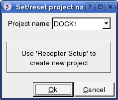
Now setup the receptor.

12.7.5 Protein-Protein Receptor Setup

Docking/Protein-protein/Receptor setup

• Enter the Docking Project name e.g. DOCK1
• Enter the receptor molecule e.g. a_2st1.m (use a_2st1.* if you want to include all molecules such as Calcium ions)
• Click OK

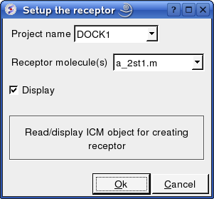
Now setup the ligand.

12.7.6 Protein-Protein Ligand Setup

Docking/Protein-protein/Ligand setup

• Enter the project name e.g. DOCK1
• Enter the ligand molecule e.g. a_2ci2.i
• If you wish to compare your docking data with a solved structure enter the name of the converted reference object in the "Reference Object" data entry box e.g. a_2sni.
• Click OK

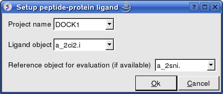
Now select an initial point of interest on the receptor referred to as epitope selection (NOTE: This step is optional. If you do not wish to select an initial point of interest junp to the make maps section. It is recommended to narrow down the docking interaction site as much as possible by selecting epitoptes. Protein-protein interaction sites can be predicted by ODA or experimental data or based on a reference complex.

12.7.7 Epitope Selection

Docking/Protein-protein/Epitope selection

Select an initial point of interest on the receptor for the docking simulation. You may want to check biological data or a reference complex or predict interaction sites using ODA before doing this step. If you do not know the docking interface location you should setup multiple docking runs for different epitopes on the receptor.

• You can make selections on either the ligand or receptor or both the ligand and receptor. Check the appropriate box(es).
• A display as shown below will be displayed.
• Using the right button of the mouse select a numbered sphere surrounding the receptor or ligand that you wish to dock to by clicking and dragging the mouse over the sphere. The spheres are numbered and change color from purple to yellow when they are selected. If you are happy with the selection type 'a' or press the apply button. The selected numbered regions will change from purple to yellow. The easiest way to select multiple epitopes is to use the pick atom button (green cross button).
• When you have finished selecting the epitoples type 'q' or select the quit button in the terminal window.

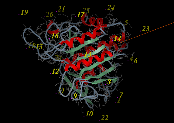
NOTE: If you are unsure which epitopes you have selected they are listed in the DOCKING_PROJECT_NAME.tab file in the first two fields called I_selLigPos (receptor epitopes) and I_selLigRot (ligand epitopes).

The next step is to make the maps of the receptor.

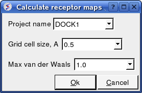
12.7.8 Protein-Protein Make Receptor Maps

Docking/Protein-protein/Make Receptor Maps

• Enter the Project name e.g. DOCK1
• Enter the grid size e.g. how detailed you want your maps - the default value of 0.5 is generally ok.
• Enter the Max van der Waals value which gives the receptor an element of 'softness' to incoporate some induced fit - the default value of 1.0 is generally ok.

Now run the docking simulation.

12.7.9 Protein-Protein Docking Batch

The docking can be run on your local machine or in PBS.

To run on your local machine:

Docking/Protein-protein/Docking Batch/Local Machine

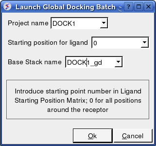
• Enter the Project Name
• Starting Position for Ligand - if you select 0 it will sample all the points on the receptor you selected in the epitope step of the docking project setup. If however you want to break your jobs down into smaller chunks you can enter the number of a position on the receptor you chose in the epitope selection step and it will sample that point.
• Enter a name for the conformational stack which will be saved.

To run in PBS:

Docking/Protein-protein/Docking Batch/PBS

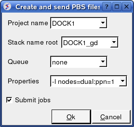
You can check the docking progress by going to Windows/Background Jobs. Once the docking has finished a dialog window will be displayed telling you that the docking job is complete - Click OK and a results table will be displayed. Read the next section on how to view the results.

Error messages are reported at the end of the DOCKING_Project.ou output file. You can also see details about any errors by clicking on the Details button in the dialog window which is displayed once the docking run is finished.

12.7.10 Display Grid Docking Results

Once the docking is finished you should see a table A table as shown below will be displayed. You can sort the table by Energy (ener) by right clicking on the column header and select sort.

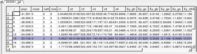
To display the complexes:

• Single click on a row of the table shown above. The ligand will be displayed in the ICM workspace and named according to the project name followed by "_lig" (e.g. DOCK1_lig).
• Check the R_Srmsd column for the difference between docked and the crystal structure complex for comparison (if selected).
• To view interactions between the receptor and the ligand each molecule needs to be in the same object. See the FAQ section: How do I merge two separate objects into one.

If no docking table is displayed you can process the results by:

• Docking/Protein-protein/Docking Batch/Process Global Docking Solutions.

The output columns represent:

• i - a slot number in the stack of conformations
• ener - total energy as calculated before the conformation was stored
• rmsd - the distance (either Cartesian or angular RMSD) between the current conformation of the object and the stack conformation calculated according to the compare command.
• naft - the number of visits AFTER the last improvement of energy
• nvis - the total number of visits to this slot; since new conformation are only compared with the last stack conformation the conformations may drift and cover a large area than described by the vicinity parameter
• v1 to v6 - are the virtual variables defining position and rotation of the ligand molecule.
• ey gh - van der Waals grid potential - hydrogen probe
• ey gc - van der Waals grid potential - carbon probe
• ey gb hydrogen bonding grid potential
• ey ge electrobstatics grid potential
• hydrophobic potential
• ey sfPola - polar terms of the solvation energy
• Ey_sfAl - aliphatic terms of the solvation energy
• Ey_sfAr - aromatic terms of the solvation energy
• Ey_compSol - weighted total of the solvation energy terms

All your docking data is saved so if you want to return to view the table at a later date please use the following commands in the command line.

read object "DOCK1_rec" # read receptor (if not read yet)
display a_DOCK1_rec.    # display receptor (if not displayed yet)
read object "DOCK1_lig" # read ligand object
display a_              # display this ligand
read table  "DOCK1_gd.Var" # read table of the ligand conformations. Click on table rows to view ligand conformations

12.7.11 Complex Refinement

You can refine a complex by:

• Right click on the conformation you wish to refine in the results table.
• Select the option Refine Conformation.
• Click the green GO button located at the bottom of the graphical user interface.

Once the simulation has finished you can view the results by:

• MolMechanics/Stack View
• A table will be displayed called confStack ranked by energy.
• Click on each row of the table to view the solution.