[ Assign Helices and Strands | Reactive Cysteine | Protein Health | Local Flexibility | Protein-Protein Interface Prediction | Identify Ligand Pockets ]
| Available in the following product(s): ICM-Pro |
Chapter Contents:
- Assign Helices and Strands
- Protein Health
- Local Flexibility
- Protein-Protein Interface Prediction
- Identfy Ligand Pockets
Theory
The Assign helices and Strands option will manually reassign secondary structure to a protein structure. This command does not change the geometry of the model, it only formally assigns secondary structure symbols to residues. The method uses a modification of the DSSP algorithm of automatic secondary structure assignment (Kabsch and Sander, 1983) based on the observed pattern of hydrogen bonds in a three dimensional structure. The DSSP algorithm in its original form overassigns the helical regions. For example, in the structure of T4 lysozyme (PDB code 103l ) DSSP assigns to one helix the whole region a_/93:112 which actually consists of two helices a_/93:105 and a_/108:112 forming a sharp angle of 64 degrees. ICM employs a modified algorithm which patches the above problem of the original DSSP algorithm.
To assign secondary structure:
- Read in a protein structure ( File/Open or PDB Search).
- Select the structure. You can do this by double clicking on the name of the structure in the ICM Workspace (a selection is highlighted blue in the ICM Workspace and green crosses in the graphical display) or you can use the right-click button and drag it over the whole structure in the graphical display.
- Tools/3D Predict/Assign helices and Strands.
The secondary structure sequence string (e.g. EEEEEEEEE__HHHH) will be displayed in the terminal window. Assigned secondary structure types are the following: "H" - alpha helix, "G" - 3/10 helix, "I" - pi helix, "E" - beta strand, "B" - beta-bridge, "_" or "C" - coil. If the sequence is viewed in the ICM workspace or in an alignment the secondary structure is colored as follows alpha helix (red bar), beta sheet (green bar), non-canonical helix (purple bar).
To predict how reactive a Cys residue is and how likely it is to form a covalent bond.
- Read into ICM a PDB or protein molecule.
- Convert your molecule to an ICM object.
- Select the cysteines you want to analyze.
- Tools/3D Predict/Reactive Cys... There are options to include ligands in the analysis and use all chains in the molecule.
- A results table will be displayed.
About the results table:
- residue = cystein residue analyzed
- distToSurface = distance to the protein surface
- saSC = solvent accessible surface area of Cys side chain
- score = reactivity score - the higher the more reactive
- pocketArea25 - pocket area if there is a binding pocket within 2.5A of a CYS residue
- nearNPlus - distance to nearest positively charged Lys and Arg residues
- nearHip - distance to nearest Hip/His/Hie
- esp1 - electrostatic potential at S(Beta) of a Cys
- hbondBB - energy of hydrogen bonds with backbone
About the Method The method predicts how reactive a CYS residue is. It is based on reactivity data for 34 reactive and 184 non-reactive cysteines from isoTOP-ABPP (isotopic tandem orthogonal proteolysis activity-based protein profiling) Ref. Backus et al. 2016, Nature, 534, 570 and a nonredundant set of PDB protein structures (resolution < 2.5 A) with covalently-modified cysteines (272 reactive). A reactivity score is made based on a weighted function of the energy and distance datareported in the results table. The prediction was built using Random Forest classification and cross validated with a test set of 20% of random data.
Theory
The protein health option calculates the energy strain of a structure in ICM. It is generally a good idea to investigate the energy strain of any protein structure before undertaking such processes as docking. It is also essential to use this tool after making a model (see Molecular Modeling) to identify strained regions within your model and then some optimization procedure can be undertaken to rectify the problems.
The protein health option calculates the relative energy of each residue for a selection and colors the selected residues by strain. This macro uses statistics obtained in the following paper Maiorov, V.N. and Abagyan, R.A. (1998) Energy strain in three-dimensional protein structures Folding and Design, 3 , 259-269.
To use the Protein Health option:
- Read in a protein structure ( File/Open or PDB Search).
- Convert your PDB structure into an ICM object.
- Make a selection of the residues you wish to analyze.
- Tools/3D Predict/Protein Health and a window as shown below will be displayed.
- The scale of the coloring can be changed by altering the value within the trimEnergy data entry box.
- Click OK and the structure will be colored according to energy strain (red - high) and a table of residue energy will be displayed in a table.
- A table and plot of Normalized energies for each amino acid in the selection will be displayed. The table is ranked and colored by residues with poor normalized energies. Click on a row in the table or plot to center in on the residue.
This option systematically samples rotamers for each residue side-chain in the input selection and uses resulting conformational ensembles to evaluate energy-weighted RMSDs for every side-chain atom. These are stored in the 'field' values on atoms and can be used for example to color the structure by side-chain flexibility. Conformational entropy for each residue side-chain is also calculated and stored in a table. If l_entropyBfactor flag is on, the atom rmsds are normalized within the residue to reflect its total conformational entropy. If l_bfactor flag is set, the bfactors are reset to the same values that are placed in the atom 'field', and occupancy is set to be inversely proportional to it ( O=1/(1+2*rmsd) )
- Read pdb file (File/Open or PDB Search Tab).
- Convert to an ICM Object.
- Tools/3D Predict/Local Flexibility
The ICM Optimal Docking Area method is a useful way of predicting likely protein-protein interaction interfaces. If you do not have mutational data or other experimental data which indicates the likely protein-protein docking site this method will be useful. This procedure can save you time during the docking procedure by focusing your docking only on areas on the receptor and ligand most likely to interact.
Theory
ODA (Optimal Docking Areas) is a new method to predict protein-protein interaction sites on protein surfaces. It identifies optimal surface patches with the lowest docking desolvation energy values as calculated by atomic solvation parameters (ASP) derived from octanol/water transfer experiments and adjusted for protein-protein docking. The predictor has been benchmarked on 66 non-homologous unbound structures, and the identified interactions points (top 10 ODA hot-spots) are correctly located in 70% of the cases (80% if we disregard NMR structures). For a description of the method see Fernandez-Recio et al Proteins (2005) 127: 9632.
To display the optimal docking area.
- Convert the PDB file to an ICM object.
- Tools/3D Predict/Protein Interface by ODA
- If you select the Residue Table option the average ODA score for each residue will be displayed in a table. The lower the number the higher the chance the residue will be involved in protein-protein interactions. Regions colored red represent low ODA score and blue represents a high score.
Theory
The ICM Pocket Finder method (1-2) uses only the protein structure for the prediction of cavities and clefts. No prior knowledge of the substrate is required. The position and size of the ligand-binding pocket are determined based on a transformation of the Lennard-Jones potential by convolution with a Gaussian kernel of a certain size, a grid map of a binding potential and construction of equipotential surfaces along the maps. The pockets are displayed graphically as a surface and the dimensions of each pocket are presented in an interactive table and plot.
Factors that can influence ligand binding to a pocket include the pocket volume and area, buriedness, hydrophobicity, and how compact the pocket is. All these properties are calculated using ICMPocketFinder and tabulated. Scientists at Merck used MolSoft.s ICMPocketFinder algorithm to define a way for quantifying "drugability" of a protein target (3). The metric they used is called Drug-Like-Density (DLID), and this score is also provided in the results table. A good example of the use of the icmPocketFinder method is in the database called Pocketome. The Pocketome (www.pocketome.org) is an encyclopedia of conformational ensembles of all druggable binding sites that can be identified experimentally from co-crystal structures in the Protein Data Bank (4).
1. An, J., Totrov, M. & Abagyan, R. Pocketome via comprehensive identification and classification of ligand binding envelopes. Mol. Cell. Proteomics 4, 752 (2005).
2. Abagyan, R. & Kufareva, I. The flexible pocketome engine for structural chemogenomics. Methods Mol. Biol. Clifton NJ 575, 249.279 (2009).
3. Sheridan, R. P., Maiorov, V. N., Holloway, M. K., Cornell, W. D. & Gao, Y.-D. Drug-like density: a method of quantifying the .bindability. of a protein target based on a very large set of pockets and drug-like ligands from the Protein Data Bank. J. Chem. Inf. Model. 50, 2029.2040 (2010).
4. Kufareva, I., Ilatovskiy, A. V. & Abagyan, R. Pocketome: an encyclopedia of small-molecule binding sites in 4D. Nucleic Acids Res. 40, D535.540 (2012).
To predict pockets:
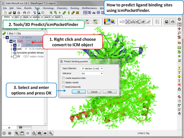 |
|
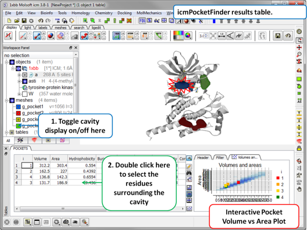 |
Results
|
About the icmPocketFinder Results Table
Factors that can influence ligand binding to a pocket include the pocket volume and area, buriedness, hydrophobicity, and how compact the pocket is. These values are reported in the results table:
- Volume of the pocket in Å.
- Area of the pocket in Å.
- Hydrophobicity - represents the percentage of the pocket surface s in contact with hydrophobic protein residues (values can range from 0-1)
- Buriedness - The buriedness parameter is calculated as follows: One measures the solvent accessible surface area of the pocket (probe radius, 1.4) in isolation. Then one measures the solvent accessible surface area of the pocket covered by its shell. The ratio of the second number to the first is the fraction buried. The lowest possible value is 0.5; i.e. the pocket is completely open and the surface flat. The highest is 1.0, i.e., completely buried.
- DLID - Merck's Drug-like density score (see Sheridan et al JCIM 2010). Values above zero and those with slightly negative values are considered "druggable".
- Loop Fraction - fraction of pocket formed by residues from loops (lower is better)
- dTSsc - Estimate of entropic penalty associated with flexible side-chains forming parts of the pocket
- relTSssc - Same as dTSssc but relative to pocket volume. (lower is better)
- Bfactor Average b-factor of pocket-forming atoms (lower is better)
- relBfactor - Normalized deviation of pocket b-factor from the average over the protein (lower is better)
- Aromatic - fraction of pocket formed by aromatic side-chains (higher is better)
- Radius gives an indication of how spherical a pocket is. ( 3/4 Volume / Pi )^1/3 , i.e. radius of an ideal spherical cavity of the same volume as a pocket blob.
- Nonsphericity give an indication of how spherical the pocket is. Area / (area of ideal spherical cavity) . It is 1.0 if the cavity is spherical
- Conservation Average conservation (%identity) of residues in contact with the pocket. Calculation is performed if multiple alignment is present and linked to the protein chain being analyzed.
- RelCons Above conservation, relative to the average over the entire chain.
- Type - returns the ICM selection for the residues forming the pocket.