[ R-Group Decomposition | Free Wilson | SAR Table | Plot R Groups | SALI | Matched Pair Analysis ]

Tutorial | Video

To decompose a library into fragments based on a Markush scaffold (opposite of R-group (Markush) enumeration ):

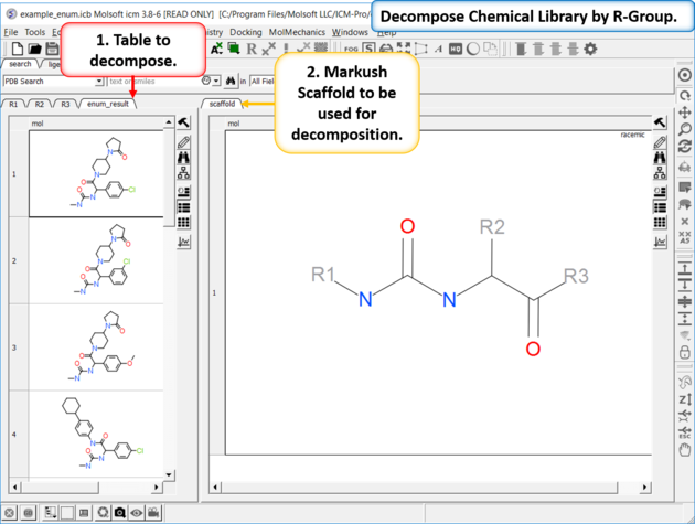
• Read the sdf file you wish to decompose into ICM and it will be displayed as a molecular table.
• Sketch the Markush structure you wish to use to decompose the table by and save it in a chemical table.

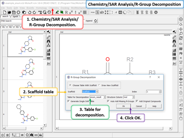
• Chemistry/SAR Analysis/R-Group Decomposition.
• Choose the table containing the Markush scaffold. Index refers to table row if you have more than one Markush structure in a table.
• Use the drop-down option to select the table you wish to decompose and the column containing the 2D chemical (usually called mol).
• If you have more than one R-group ICM can either generate a different table for each R-group or it can merge it into one single table whereby column will represent R1 and column two R2... This option is useful if you want to generate a SAR table with a column of activity data next to the R1 and R2 columns.
• If you check the box "Auto Add Missing R Groups" then unique R-groups will be extracted from the scaffold where hydrogens can be attached.

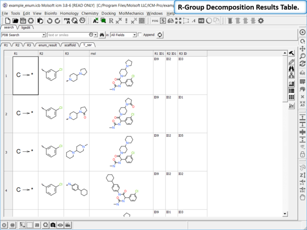
• The decomposed table will be reported in a new table with new columns for the R groups (R1,R2...). If you have an additional column with activity data you can sort the table by R-groups and see the effect of an R-Group on activity. This table can be used to build an additional SAR table as described here.

The method is based on this paper by Free and Wilson J. Med. Chem 1964.

Building a Linear Model for R-Group Decomposition and Activity Prediction

Input:

• A chemical table where molecules are decomposed into R-groups.
• An activity column containing experimental or predicted values.

Processing Steps:

1. Unique Numbering of R-Groups

Each R-group from the input set is assigned a unique identifier.

2. Descriptor Vector Formation

For each compound, a descriptor vector X[i] is created:

• 1 - The R-group is present in that row.
• 0 - The R-group is absent.

3. Linear Model Training

A Partial Least Squares (PLS) regression model is trained in MolSoft ICM.

The model uses the descriptor matrix (X) and the activity column to learn the relationship.

4. Equation Representation

The model outputs weights (W) and a bias (B) to define the equation:

Activity = X · W + B

• W - A vector of weights representing the contribution of each R-group.
• X - A matrix containing descriptor values.
• B - A scalar bias term adjusting the overall prediction.

How to run Free Wilson in ICM:

• First you need to decompose your hits using a common Markush structure to obtain a set of R-Groups.
• Chemistry/SAR Analysis/Free Wilson Regression Analysis.
• Check the option to enumerate the full library to identify promising combinations of substituents that have not yet been synthesized. This will generate all possible combinations of the available substituents. However, please note that if you have multiple R-groups with numerous potential variations, this process can produce a large number of molecules. You will see a message in the ICM terminal window if the libray is too big for the memory of your computer. It is recommended to just keep the top 1000 hits and depending on the data you are trying to predict in activity column choose 'high' or 'low' (e.g high for pKd or low for IC50).
• Enter the name of your R-Group table
• Choose the activity column and run the analysis.

Results

The results comprise the following:

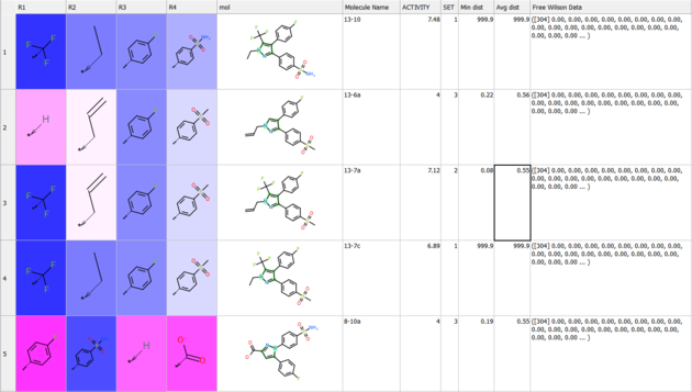
• The method assigns weights to the original SAR table under R_group_weights and highlights them:
  • Blue indicates a positive contribution to the predicted property.
  • Red indicates a negative contribution.
• Separate tables are provided for each table, making it easier to:
  • Sort the data by weight of R-group (column 'w').
  • Identify which groups have the most significant influence at specific positions.
• A model is generated and displayed in the ICM Workspace.
  • You can save the model.
  • You can apply it to other chemicals in the same series using predict.
• If the enumeration option is selected:
  • A fully enumerated library will be available.

Guide to the Free Wilson Results Table

The Free Wilson Results table provides key statistical outputs from a Free Wilson analysis using PLS (Partial Least Squares) regression. The following columns are included in the output:

• mean: Displays the average value of the response variable (e.g., biological activity) across all compounds in the dataset. This value represents the central tendency of the measured response.
• rmsd: The Root Mean Square Deviation (RMSD) measures the difference between the predicted and observed values. It quantifies the error or variance in the model's predictions, providing insight into the model's accuracy.
• corrY: The correlation coefficient between the predicted and observed values of the response variable. A high correlation indicates a strong fit between the model and the observed data.
• wCvRmsd: The weighted or cross-validation RMSD, which incorporates weighting factors or cross-validation procedures to assess model performance. It is a more robust measure of predictive accuracy.
• w: The regression weights (coefficients) derived from the Free Wilson model. These weights represent the contribution of each descriptor or feature to the predicted value, showing the influence of different chemical fragments or features.
• wRel: The relative importance of each regression weight (w). This column indicates which features (descriptors) have the most significant impact on the model, helping to identify key determinants of the predicted property.

These results are used to interpret the model's performance and understand the contributions of individual features in predicting biological responses based on chemical structures.

| Tutorial |

To generate a SAR table you first need to decompose the table into the R-Groups.

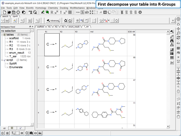Decompose your library. Decompose the library to extract the R-Groups or read in a decomposed SDF file.

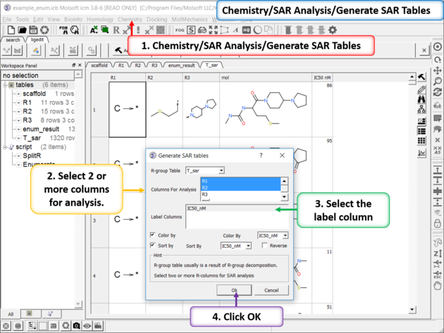Generate SAR table. Chemistry/SAR Analysis/Generate SAR Tables. One or more columns can be chosen for analysis and multiple tables will be generated. Color the table by a selected column e.g. activity.

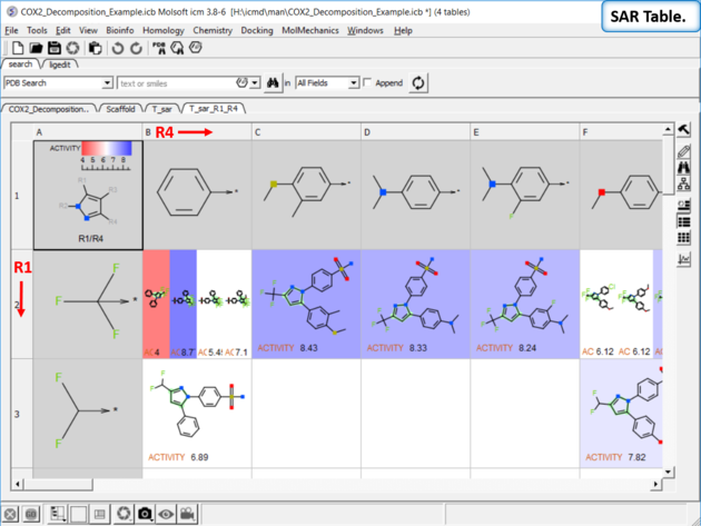SAR table. The SAR table will be displayed with an activity scale and R-group scaffold in the first cell (A1) and the R groups along each axis. You can use the table to investigate which R-group(s) contribute to activity.

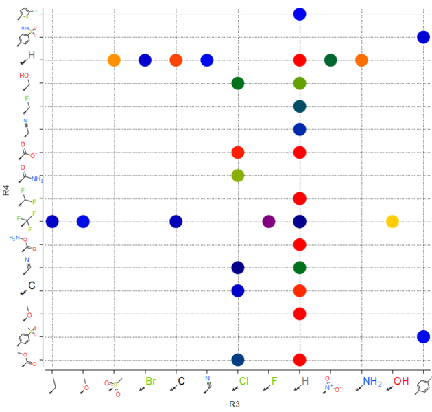
You can make a plot of R-groups from library decomposition. This is described in the plots section of the manual.

| Tutorial |

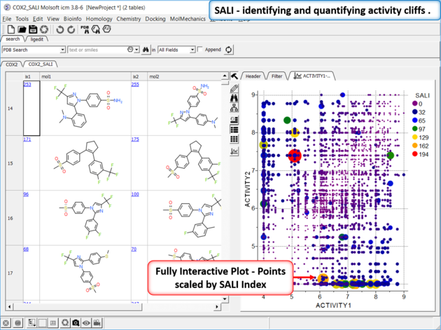
Structure--activity landscape index: identifying and quantifying activity cliffs.

This method produces a SALI score as described in the publications by John Van Drie and co-workers. It will identify "structure-activity cliffs": pairs of molecules which are most similar but have the largest change in activity.

• Read in a sdf file containing "mol" and "activity" column.
• Chemistry/SAR Analysis/Generate SALI table.
• You can choose to use the Log of the Activity Column.
• The method will try to find pairs based on defined distance cutoff (0.15 is a good threshold for larger datasets).
• A results table will be reported containing the pairs, tanimoto fingerprint similarity and SALI index.

| Tutorial |

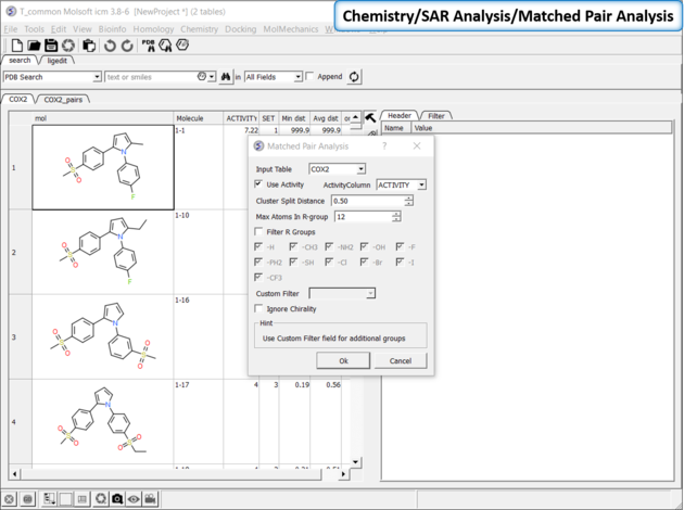
Matched Pair Analysis (MPA)can be used to study changes in chemical properties based on small well-defined structural modifications to the chemical structure. The method tries to find the Maximum Common Substructure and clusters by similarity. The analysis is performed in two stages: clustering and then Maximum common substructure on each pair in each cluster. The output is similar to SALI output plus it gives the actual R-group pair variation. The pair table is sorted by score so top hits should show small variations and big score difference. To run MPA:

Read in a chemical spreadsheet containing a 'mol' column and activity data. Chemistry/SAR Analysis/Matched Pair Analysis. Enter the name of the Input Table. If the table has activity data or some other property use the option use Activity and select the column name from the drop down button. Enter a cluster split distance for determining similarity. The size of the R-groups for comparison can be set (default is 12 atoms). R-groups can be filtered from the analysis, or by a custom filter using SMARTs. Chirality can be ignored in the comparison if needed.

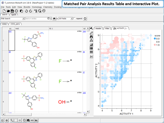The results table (tableName_pairs) is fully interactive between the plot and the original table. The hits are sorted by the score column, so top hits should show biggest activity change with smaller groups. The plot is displayed activity 1 versus activity 2 colored and sized by score (red is better). ix1 - index number (row number) of first chemical which is hyperlinked to original table. mol1 - 2D structure of first chemical. R1_1 - group difference between first (ix1) and second chemical (ix2). ix2 - index number (row number) of second chemical which is hyperlinked to original table. mol2 2D structure of second chemical. R1_2 - group difference between second (ix2) and first chemical (ix1). scfl - common scaffold dvisible ('d' delta 'visible' - delta of your activity column: 'd' + original_column_name) score is calculated as normalized dActivity + (1 - normalized weight of both groups).